VMAT#
Overview#
The VMAT module consists of the class VMAT, which is capable of loading an EPID DICOM Open field image and MLC field image and analyzing the images according to the Varian RapidArc QA tests and procedures, specifically the Dose-Rate & Gantry-Speed (DRGS) and Dose-Rate & MLC speed (DRMLC) tests.
Features:
Do both tests - Pylinac can handle either DRGS or DRMLC tests.
Automatic offset correction - Older VMAT tests had the ROIs offset, newer ones are centered. No worries, pylinac finds the ROIs automatically.
Automatic open/DMLC identification - Pass in both images–don’t worry about naming. Pylinac will automatically identify the right images.
Note
There are two classes in the VMAT module: DRGS and DRMLC. Each have the exact same methods.
Anytime one class is used here as an example, the other class can be used the same way.
Running the Demos#
For this example we will use the DRGS class:
from pylinac import DRGS
DRGS.run_demo()
(Source code, png, hires.png, pdf)

Results will be printed to the console and a figure showing both the Open field and MLC field image will pop up:
Dose Rate & Gantry Speed
Test Results (Tol. +/-1.5%): PASS
Max Deviation: 1.01%
Absolute Mean Deviation: 0.459%
Image Acquisition#
If you want to perform these specific QA tests, you’ll need DICOM plan files that control the linac precisely to deliver the test fields. These can be downloaded from my.varian.com. Once logged in, search for RapidArc and you should see two items called “RapidArc QA Test Procedures and Files for TrueBeam”; there will be a corresponding one for C-Series. Use the RT Plan files and follow the instructions, not including the assessment procedure, which is the point of this module. Save & move the VMAT images to a place you can use pylinac.
Typical Use#
The VMAT QA analysis follows what is specified in the Varian RapidArc QA tests and assumes your tests will run the exact same way. Import the appropriate class:
from pylinac import DRGS, DRMLC
The minimum needed to get going is to:
Load images – Loading the EPID DICOM images into your VMAT class object can be done by passing the file paths, passing a ZIP archive, or passing a URL:
open_img = "C:/QA Folder/VMAT/open_field.dcm"
dmlc_img = "C:/QA Folder/VMAT/dmlc_field.dcm"
mydrgs = DRGS(image_paths=(open_img, dmlc_img))  # use the DRMLC class the exact same way

# from zip
mydrmlc = DRMLC.from_zip(r'C:/path/to/zip.zip')

# from a URL
mydrgs = DRGS.from_url('http://myserver.org/vmat.zip')
Finally, if you don’t have any images, you can use the demo ones provided:
mydrgs = DRGS.from_demo_images()
mydrmlc = DRMLC.from_demo_images()
Analyze the images – Once the images are loaded, tell the class to analyze the images. See the Algorithm section for details on how this is done. Tolerance can also be passed and has a default value of 1.5%:
mydrgs.analyze(tolerance=1.5)
View/Save the results – The VMAT module can print out the summary of results to the console as well as draw a matplotlib image to show where the segments were placed and their values:
# print results to the console
print(mydrgs.results())
# view analyzed images
mydrgs.plot_analyzed_image()
(
Source code,png,hires.png,pdf)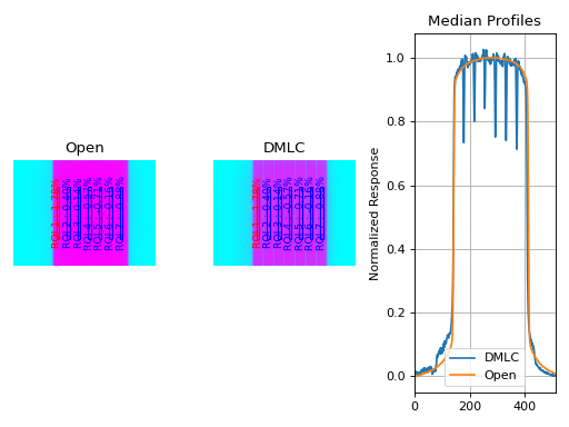
PDF reports can also be generated:
myvmat.publish_pdf('drgs.pdf')
Customizing the analysis#
You can alter both the segment size and segment positions as desired.
To change the segment size:
drgs = DRGS.from_demo_image()
drgs.analyze(..., segment_size_mm=(10, 150))  # ROI segments will now be 10mm wide by 150mm tall
# same story for DRMLC
To change the x-positions of the ROI segments or change the number of ROI, use a custom ROI config dictionary and pass it to the analyze method.
from pylinac import DRGS, DRMLC

# note the keys are the names of the ROIs and can be anything you like
custom_roi_config = {'200 MU/min': {'offset_mm': -100}, '300 MU/min': {'offset_mm': -80}, ...}

my_drgs = DRGS(...)  # works the same way for DRMLC
my_drgs.analyze(..., roi_config=custom_roi_config)
(Source code, png, hires.png, pdf)

Accessing Data#
Changed in version 3.0.
Using the VMAT module in your own scripts? While the analysis results can be printed out,
if you intend on using them elsewhere (e.g. in an API), they can be accessed the easiest by using the results_data() method
which returns a VMATResult instance.
Note
While the pylinac tooling may change under the hood, this object should remain largely the same and/or expand. Thus, using this is more stable than accessing attrs directly.
Continuing from above:
data = my_drmlc.results_data()
data.test_type
data.passed
# and more

# return as a dict
data_dict = my_drmlc.results_data(as_dict=True)
data_dict['test_type']
...
Algorithm#
The VMAT analysis algorithm is based on the Varian RapidArc QA Test Procedures for C-Series and Truebeam. Two tests (besides Picket Fence, which has its own module) are specified. Each test takes 10x0.5cm samples, each corresponding to a distinct section of radiation. A corrected reading of each segment is made, defined as: \(M_{corr}(x) = \frac{M_{DRGS}(x)}{M_{open}(x)} * 100\). The reading deviation of each segment is calculated as: \(M_{deviation}(x) = \frac{M_{corr}(x)}{M_{corr}} * 100 - 100\), where \(M_{corr}\) is the average of all segments.
The algorithm works like such:
Allowances
The images can be acquired at any SID.
The images can be acquired with any EPID (aS500, aS1000, aS1200).
Restrictions
Warning
Analysis can fail or give unreliable results if any Restriction is violated.
The tests must be delivered using the DICOM RT plan files provided by Varian which follow the test layout of Ling et al.
The images must be acquired with the EPID.
Pre-Analysis
Determine image scaling – Segment determination is based on offsets from the center pixel of the image. However, some physicists use 150 cm SID and others use 100 cm, and others can use a clinical setting that may be different than either of those. To account for this, the SID is determined and then scaling factors are determined to be able to perform properly-sized segment analysis.
Analysis
Note
Calculations tend to be lazy, computed only on demand. This represents a nominal analysis where all calculations are performed.
Calculate sample boundaries – The Segment x-positions are based on offsets from the center of the FWHM of the detected field. This allows for old and new style tests that have an x-offset from each other. These values are then scaled with the image scaling factor determined above.
Calculate the corrected reading – For each segment, the mean pixel value is determined for both the open and DMLC image. These values are used to determine the corrected reading: \(M_{corr}\).
Calculate sample and segment ratios – The sample values of the DMLC field are divided by their corresponding open field values.
Calculate segment deviations – Segment deviation is then calculated once all the corrected readings are determined. The average absolute deviation is also calculated.
Post-Analysis
Test if segments pass tolerance – Each segment is checked to see if it was within the specified tolerance. If any samples fail, the whole test is considered failing.
Benchmarking the Algorithm#
With the image generator module we can create test images to test the VMAT algorithm on known results. This is useful to isolate what is or isn’t working if the algorithm doesn’t work on a given image and when commissioning pylinac.
Note
The below examples are for the DRMLC test but can equally be applied to the DRGS tests as well.
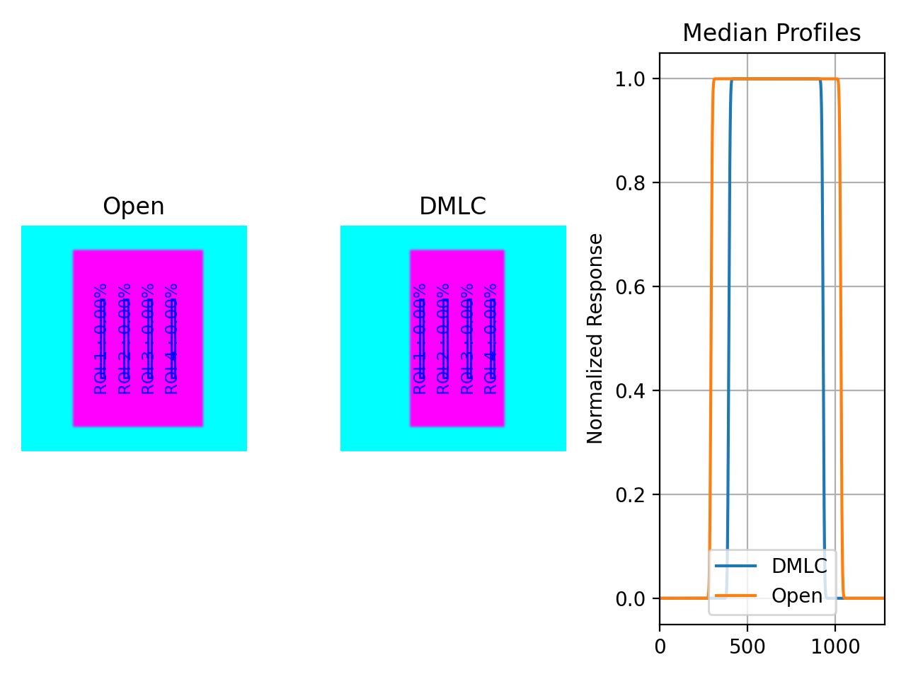
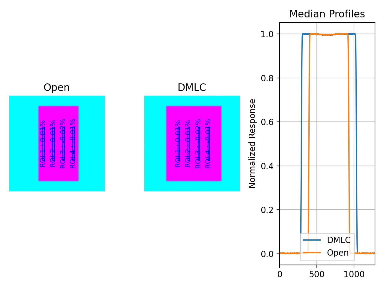
Perfect Fields#
In this example, we generate a perfectly flat set of images.
The script will generate the files, but you can also download them here:
perfect_open_drmlc.dcm perfect_dmlc_drmlc.dcm.
import pylinac
from pylinac.core.image_generator import GaussianFilterLayer, PerfectFieldLayer, AS1200Image

# open image
open_path = 'perfect_open_drmlc.dcm'
as1200 = AS1200Image()
as1200.add_layer(PerfectFieldLayer(field_size_mm=(150, 110), cax_offset_mm=(0, 5)))
as1200.add_layer(GaussianFilterLayer(sigma_mm=2))
as1200.generate_dicom(file_out_name=open_path)

# DMLC image
dmlc_path = 'perfect_dmlc_drmlc.dcm'
as1200 = AS1200Image()
for offset in (-40, -10, 20, 50):
    as1200.add_layer(PerfectFieldLayer((150, 20), cax_offset_mm=(0, offset)))
as1200.add_layer(GaussianFilterLayer(sigma_mm=2))
as1200.generate_dicom(file_out_name=dmlc_path)

# analyze it
vmat = pylinac.DRMLC(image_paths=(open_path, dmlc_path))
vmat.analyze()
print(vmat.results())
vmat.plot_analyzed_image()
(Source code, png, hires.png, pdf)
with output:
Dose Rate & MLC Speed
Test Results (Tol. +/-1.5%): PASS
Max Deviation: 0.0%
Absolute Mean Deviation: 0.0%
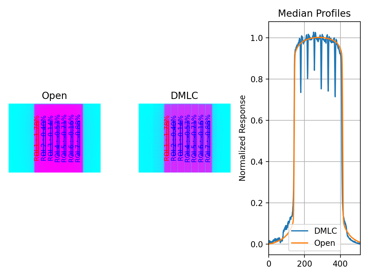
Noisy, Realistic#
We now add a horn effect and random noise to the data:
import pylinac
from pylinac.core.image_generator import GaussianFilterLayer, FilteredFieldLayer, AS1200Image, RandomNoiseLayer

# open image
open_path = 'noisy_open_drmlc.dcm'
as1200 = AS1200Image()
as1200.add_layer(FilteredFieldLayer(field_size_mm=(150, 110), cax_offset_mm=(0, 5)))
as1200.add_layer(GaussianFilterLayer(sigma_mm=2))
as1200.add_layer(RandomNoiseLayer(sigma=0.03))
as1200.generate_dicom(file_out_name=open_path)

# DMLC image
dmlc_path = 'noisy_dmlc_drmlc.dcm'
as1200 = AS1200Image()
for offset in (-40, -10, 20, 50):
    as1200.add_layer(FilteredFieldLayer((150, 20), cax_offset_mm=(0, offset)))
as1200.add_layer(GaussianFilterLayer(sigma_mm=2))
as1200.add_layer(RandomNoiseLayer(sigma=0.03))
as1200.generate_dicom(file_out_name=dmlc_path)

# analyze it
vmat = pylinac.DRMLC(image_paths=(open_path, dmlc_path))
vmat.analyze()
print(vmat.results())
vmat.plot_analyzed_image()
(Source code, png, hires.png, pdf)
with output:
Dose Rate & MLC Speed
Test Results (Tol. +/-1.5%): PASS
Max Deviation: 0.0332%
Absolute Mean Deviation: 0.0257%
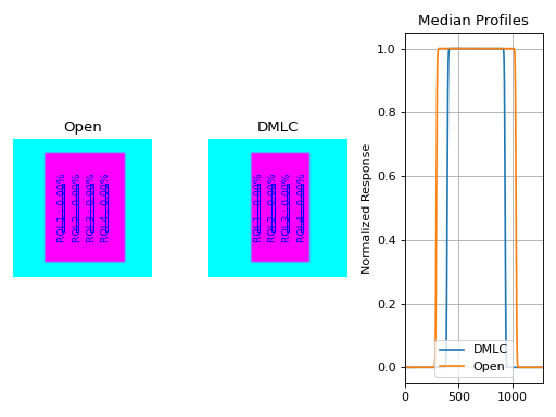
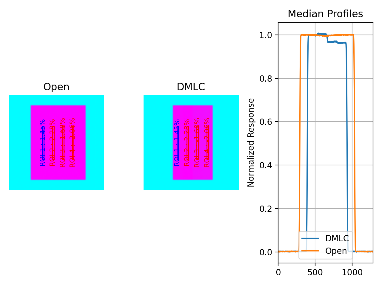
Erroneous data#
Let’s now get devious and randomly adjust the height of each ROI (effectively changing the apparent MLC speed):
Note
Due to the purposely random nature shown below, this exact result is likely not reproducible, nor was it intended to be. To get reproducible behavior, use numpy with a seed value.
import random

import pylinac
from pylinac.core.image_generator import GaussianFilterLayer, FilteredFieldLayer, AS1200Image, RandomNoiseLayer

# open image
open_path = 'noisy_open_drmlc.dcm'
as1200 = AS1200Image()
as1200.add_layer(FilteredFieldLayer(field_size_mm=(150, 110), cax_offset_mm=(0, 5)))
as1200.add_layer(GaussianFilterLayer(sigma_mm=2))
as1200.add_layer(RandomNoiseLayer(sigma=0.03))
as1200.generate_dicom(file_out_name=open_path)

# DMLC image
dmlc_path = 'noisy_dmlc_drmlc.dcm'
as1200 = AS1200Image()
for offset in (-40, -10, 20, 50):
    as1200.add_layer(FilteredFieldLayer((150, 20), cax_offset_mm=(0, offset), alpha=random.uniform(0.93, 1)))
as1200.add_layer(GaussianFilterLayer(sigma_mm=2))
as1200.add_layer(RandomNoiseLayer(sigma=0.03))
as1200.generate_dicom(file_out_name=dmlc_path)

# analyze it
vmat = pylinac.DRMLC(image_paths=(open_path, dmlc_path))
vmat.analyze()
print(vmat.results())
vmat.plot_analyzed_image()
(Source code, png, hires.png, pdf)
with an output of:
Dose Rate & MLC Speed
Test Results (Tol. +/-1.5%): FAIL
Max Deviation: 2.12%
Absolute Mean Deviation: 1.13%
API Documentation#
Main classes#
These are the classes a typical user may interface with.
- class pylinac.vmat.DRGS(image_paths: Sequence[str | BinaryIO | Path])[source]#
Class representing a Dose-Rate, Gantry-speed VMAT test. Will accept, analyze, and return the results.
- Parameters:
image_paths (iterable (list, tuple, etc)) – A sequence of paths to the image files.
- analyze(tolerance: float | int = 1.5, segment_size_mm: tuple = (5, 100), roi_config: dict | None = None)#
Analyze the open and DMLC field VMAT images, according to 1 of 2 possible tests.
- Parameters:
tolerance (float, int, optional) – The tolerance of the sample deviations in percent. Default is 1.5. Must be between 0 and 8.
segment_size_mm (tuple(int, int)) – The (width, height) of the ROI segments in mm.
roi_config (dict) – A dict of the ROI settings. The keys are the names of the ROIs and each value is a dict containing the offset in mm ‘offset_mm’.
- property avg_abs_r_deviation: float#
Return the average of the absolute R_deviation values.
- property avg_r_deviation: float#
Return the average of the R_deviation values, including the sign.
- classmethod from_demo_images()#
Construct a VMAT instance using the demo images.
- classmethod from_url(url: str)#
Load a ZIP archive from a URL. Must follow the naming convention.
- Parameters:
url (str) – Must point to a valid URL that is a ZIP archive of two VMAT images.
- classmethod from_zip(path: str | Path)#
Load VMAT images from a ZIP file that contains both images. Must follow the naming convention.
- Parameters:
path (str) – Path to the ZIP archive which holds the VMAT image files.
- property max_r_deviation: float#
Return the value of the maximum R_deviation segment.
- plot_analyzed_image(show: bool = True, show_text: bool = True, **plt_kwargs: dict)#
Plot the analyzed images. Shows the open and dmlc images with the segments drawn; also plots the median profiles of the two images for visual comparison.
- Parameters:
show (bool) – Whether to actually show the image.
show_text (bool) – Whether to show the ROI names on the image.
plt_kwargs (dict) – Keyword args passed to the plt.subplots() method. Allows one to set things like figure size.
- publish_pdf(filename: str, notes: str = None, open_file: bool = False, metadata: dict | None = None, logo: Path | str | None = None)#
Publish (print) a PDF containing the analysis, images, and quantitative results.
- Parameters:
filename ((str, file-like object}) – The file to write the results to.
notes (str, list of strings) – Text; if str, prints single line. If list of strings, each list item is printed on its own line.
open_file (bool) – Whether to open the file using the default program after creation.
metadata (dict) – Extra data to be passed and shown in the PDF. The key and value will be shown with a colon. E.g. passing {‘Author’: ‘James’, ‘Unit’: ‘TrueBeam’} would result in text in the PDF like: ————– Author: James Unit: TrueBeam ————–
logo (Path, str) – A custom logo to use in the PDF report. If nothing is passed, the default pylinac logo is used.
- property r_devs: ndarray#
Return the deviations of all segments as an array.
- results() str#
A string of the summary of the analysis results.
- Returns:
The results string showing the overall result and deviation statistics by segment.
- Return type:
str
- results_data(as_dict=False) VMATResult | dict#
Present the results data and metadata as a dataclass or dict. The default return type is a dataclass.
- class pylinac.vmat.DRMLC(image_paths: Sequence[str | BinaryIO | Path])[source]#
Class representing a Dose-Rate, MLC speed VMAT test. Will accept, analyze, and return the results.
- Parameters:
image_paths (iterable (list, tuple, etc)) – A sequence of paths to the image files.
- analyze(tolerance: float | int = 1.5, segment_size_mm: tuple = (5, 100), roi_config: dict | None = None)#
Analyze the open and DMLC field VMAT images, according to 1 of 2 possible tests.
- Parameters:
tolerance (float, int, optional) – The tolerance of the sample deviations in percent. Default is 1.5. Must be between 0 and 8.
segment_size_mm (tuple(int, int)) – The (width, height) of the ROI segments in mm.
roi_config (dict) – A dict of the ROI settings. The keys are the names of the ROIs and each value is a dict containing the offset in mm ‘offset_mm’.
- property avg_abs_r_deviation: float#
Return the average of the absolute R_deviation values.
- property avg_r_deviation: float#
Return the average of the R_deviation values, including the sign.
- classmethod from_demo_images()#
Construct a VMAT instance using the demo images.
- classmethod from_url(url: str)#
Load a ZIP archive from a URL. Must follow the naming convention.
- Parameters:
url (str) – Must point to a valid URL that is a ZIP archive of two VMAT images.
- classmethod from_zip(path: str | Path)#
Load VMAT images from a ZIP file that contains both images. Must follow the naming convention.
- Parameters:
path (str) – Path to the ZIP archive which holds the VMAT image files.
- property max_r_deviation: float#
Return the value of the maximum R_deviation segment.
- plot_analyzed_image(show: bool = True, show_text: bool = True, **plt_kwargs: dict)#
Plot the analyzed images. Shows the open and dmlc images with the segments drawn; also plots the median profiles of the two images for visual comparison.
- Parameters:
show (bool) – Whether to actually show the image.
show_text (bool) – Whether to show the ROI names on the image.
plt_kwargs (dict) – Keyword args passed to the plt.subplots() method. Allows one to set things like figure size.
- publish_pdf(filename: str, notes: str = None, open_file: bool = False, metadata: dict | None = None, logo: Path | str | None = None)#
Publish (print) a PDF containing the analysis, images, and quantitative results.
- Parameters:
filename ((str, file-like object}) – The file to write the results to.
notes (str, list of strings) – Text; if str, prints single line. If list of strings, each list item is printed on its own line.
open_file (bool) – Whether to open the file using the default program after creation.
metadata (dict) – Extra data to be passed and shown in the PDF. The key and value will be shown with a colon. E.g. passing {‘Author’: ‘James’, ‘Unit’: ‘TrueBeam’} would result in text in the PDF like: ————– Author: James Unit: TrueBeam ————–
logo (Path, str) – A custom logo to use in the PDF report. If nothing is passed, the default pylinac logo is used.
- property r_devs: ndarray#
Return the deviations of all segments as an array.
- results() str#
A string of the summary of the analysis results.
- Returns:
The results string showing the overall result and deviation statistics by segment.
- Return type:
str
- results_data(as_dict=False) VMATResult | dict#
Present the results data and metadata as a dataclass or dict. The default return type is a dataclass.
- class pylinac.vmat.VMATResult(test_type: str, tolerance_percent: float, max_deviation_percent: float, abs_mean_deviation: float, passed: bool, segment_data: Iterable[SegmentResult], named_segment_data: dict[str, pylinac.vmat.SegmentResult])[source]#
This class should not be called directly. It is returned by the
results_data()method. It is a dataclass under the hood and thus comes with all the dunder magic.Use the following attributes as normal class attributes.
- test_type: str#
- tolerance_percent: float#
- max_deviation_percent: float#
- abs_mean_deviation: float#
- passed: bool#
- segment_data: Iterable[SegmentResult]#
- named_segment_data: dict[str, SegmentResult]#
Supporting Classes#
You generally won’t have to interface with these unless you’re doing advanced behavior.
- class pylinac.vmat.VMATBase(image_paths: Sequence[str | BinaryIO | Path])[source]#
- Parameters:
image_paths (iterable (list, tuple, etc)) – A sequence of paths to the image files.
- classmethod from_url(url: str)[source]#
Load a ZIP archive from a URL. Must follow the naming convention.
- Parameters:
url (str) – Must point to a valid URL that is a ZIP archive of two VMAT images.
- classmethod from_zip(path: str | Path)[source]#
Load VMAT images from a ZIP file that contains both images. Must follow the naming convention.
- Parameters:
path (str) – Path to the ZIP archive which holds the VMAT image files.
- analyze(tolerance: float | int = 1.5, segment_size_mm: tuple = (5, 100), roi_config: dict | None = None)[source]#
Analyze the open and DMLC field VMAT images, according to 1 of 2 possible tests.
- Parameters:
tolerance (float, int, optional) – The tolerance of the sample deviations in percent. Default is 1.5. Must be between 0 and 8.
segment_size_mm (tuple(int, int)) – The (width, height) of the ROI segments in mm.
roi_config (dict) – A dict of the ROI settings. The keys are the names of the ROIs and each value is a dict containing the offset in mm ‘offset_mm’.
- results() str[source]#
A string of the summary of the analysis results.
- Returns:
The results string showing the overall result and deviation statistics by segment.
- Return type:
str
- results_data(as_dict=False) VMATResult | dict[source]#
Present the results data and metadata as a dataclass or dict. The default return type is a dataclass.
- property r_devs: ndarray#
Return the deviations of all segments as an array.
- property avg_abs_r_deviation: float#
Return the average of the absolute R_deviation values.
- property avg_r_deviation: float#
Return the average of the R_deviation values, including the sign.
- property max_r_deviation: float#
Return the value of the maximum R_deviation segment.
- plot_analyzed_image(show: bool = True, show_text: bool = True, **plt_kwargs: dict)[source]#
Plot the analyzed images. Shows the open and dmlc images with the segments drawn; also plots the median profiles of the two images for visual comparison.
- Parameters:
show (bool) – Whether to actually show the image.
show_text (bool) – Whether to show the ROI names on the image.
plt_kwargs (dict) – Keyword args passed to the plt.subplots() method. Allows one to set things like figure size.
- publish_pdf(filename: str, notes: str = None, open_file: bool = False, metadata: dict | None = None, logo: Path | str | None = None)[source]#
Publish (print) a PDF containing the analysis, images, and quantitative results.
- Parameters:
filename ((str, file-like object}) – The file to write the results to.
notes (str, list of strings) – Text; if str, prints single line. If list of strings, each list item is printed on its own line.
open_file (bool) – Whether to open the file using the default program after creation.
metadata (dict) – Extra data to be passed and shown in the PDF. The key and value will be shown with a colon. E.g. passing {‘Author’: ‘James’, ‘Unit’: ‘TrueBeam’} would result in text in the PDF like: ————– Author: James Unit: TrueBeam ————–
logo (Path, str) – A custom logo to use in the PDF report. If nothing is passed, the default pylinac logo is used.
- class pylinac.vmat.Segment(center_point: Point, open_image: image.DicomImage, dmlc_image: image.DicomImage, tolerance: float | int)[source]#
A class for holding and analyzing segment data of VMAT tests.
For VMAT tests, there are either 4 or 7 ‘segments’, which represents a section of the image that received radiation under the same conditions.
- r_dev#
The reading deviation (R_dev) from the average readings of all the segments. See documentation for equation info.
- Type:
float
- r_corr#
The corrected reading (R_corr) of the pixel values. See documentation for explanation and equation info.
- Type:
float
- passed#
Specifies where the segment reading deviation was under tolerance.
- Type:
boolean
- Parameters:
width (number) – Width of the rectangle. Must be positive
height (number) – Height of the rectangle. Must be positive.
center (Point, iterable, optional) – Center point of rectangle.
as_int (bool) – If False (default), inputs are left as-is. If True, all inputs are converted to integers.
- property r_corr: float#
Return the ratio of the mean pixel values of DMLC/OPEN images.
- property passed: bool#
Return whether the segment passed or failed.
- get_bg_color() str[source]#
Get the background color of the segment when plotted, based on the pass/fail status.
- plot2axes(axes: Axes, edgecolor: str = 'black', angle: float = 0.0, fill: bool = False, alpha: float = 1, facecolor: str = 'g', label=None, text: str = '', fontsize: str = 'medium', text_rotation: float = 0)#
Plot the Rectangle to the axes.
- Parameters:
axes (matplotlib.axes.Axes) – An MPL axes to plot to.
edgecolor (str) – The color of the circle.
angle (float) – Angle of the rectangle.
fill (bool) – Whether to fill the rectangle with color or leave hollow.
text (str) – If provided, plots the given text at the center. Useful for identifying ROIs on a plotted image apart.
fontsize (str) – The size of the text, if provided. See https://matplotlib.org/stable/api/_as_gen/matplotlib.pyplot.text.html for options.
text_rotation (float) – The rotation of the text in degrees.