Custom Image Metrics#
New in version 3.16.
Pylinac images can now have arbitrary metrics calculated on them, similar to profiles. This can be useful for calculating and finding values and regions of interest in images. The system is quite flexible and allows for any number of metrics to be calculated on an image. Furthermore, this allows for re-usability of metrics, as they can be applied to any image.
Use Cases#
Calculate the mean pixel value of an area of an image.
Finding an object in the image.
Calculating the distance between two objects in an image.
Basic Usage#
To calculate metrics on an image, simply pass the metric(s) to the compute method of the image:
from pylinac.core.image import DicomImage
from pylinac.core.metrics import DiskLocator, DiskRegion

img = DicomImage("my_image.dcm")
metric = img.compute(
    metrics=DiskLocator(
        expected_position=(100, 100),
        search_window=(30, 30),
        radius=10,
        radius_tolerance=2,
    )
)
print(metric)
You may compute multiple metrics by passing a list of metrics:
from pylinac.core.image import DicomImage
from pylinac.core.metrics import DiskLocator, DiskRegion

img = DicomImage("my_image.dcm")
metrics = img.compute(
    metrics=[
        # disk 1
        DiskLocator(
            expected_position=(100, 100),
            search_window=(30, 30),
            radius=10,
            radius_tolerance=2,
        ),
        # disk 2
        DiskLocator(
            expected_position=(200, 200),
            search_window=(30, 30),
            radius=10,
            radius_tolerance=2,
        ),
    ]
)
print(metrics)
Metrics might have something to plot on the image. If so, the plot method of the image will plot the metric(s) on the image:
from pylinac.core.image import DicomImage
from pylinac.core.metrics import DiskLocator, DiskRegion

img = DicomImage("my_image.dcm")
metrics = img.compute(
    metrics=[
        # disk 1
        DiskLocator(
            expected_position=(100, 100),
            search_window=(30, 30),
            radius=10,
            radius_tolerance=2,
        ),
        # disk 2
        DiskLocator(
            expected_position=(200, 200),
            search_window=(30, 30),
            radius=10,
            radius_tolerance=2,
        ),
    ]
)
img.plot()  # plots the image with the BB positions overlaid
Built-in Metrics#
Out of the box, only two metrics currently exists, although they are useful for a number of situations:
DiskLocator and DiskRegion.
These metrics will find disks, usually BBs, in an image and then return the location or region properties.
Note
The values provided below are in pixels. The following sections show how variants of how to use the metrics using physical units and relative to the center of the image.
For example:
from pylinac.core.image import DicomImage
from pylinac.core.metrics import DiskLocator, DiskRegion

img = DicomImage("my_image.dcm")
img.compute(
    metrics=[
        DiskLocator(
            expected_position=(100, 100),
            search_window=(30, 30),
            radius=10,
            radius_tolerance=2,
        )
    ]
)
img.plot()
This will search for a disk (BB) in the image at the expected position and window size for a disk of a given radius and tolerance.
If the disk is found, the location will be returned as a Point object.
If the disk is not found, a ValueError will be raised.
The DiskRegion metric is similar, but instead of returning the location, it returns a
scikit-image regionprops object that is the region of the disk.
This allows one to then calculate things like the weighted centroid, area, etc.
Using physical units#
While pixels are useful, it is sometimes easier to use physical units.
To perform the same Disk/BB location using mm instead of pixels:
from pylinac.core.image import DicomImage
from pylinac.core.metrics import DiskLocator, DiskRegion

img = DicomImage("my_image.dcm")
img.compute(
    metrics=[
        # these are all in mm
        DiskLocator.from_physical(
            expected_position_mm=(30, 30),
            search_window_mm=(10, 10),
            radius_mm=4,
            radius_tolerance_mm=2,
        )
    ]
)
img.plot()
Relative to center#
We can also specify the expected position relative to the center of the image.
Important
We can do this using pixels OR physical units.
This will look for the disk/BB 30 pixels right and 30 pixels down from the center of the image:
from pylinac.core.image import DicomImage
from pylinac.core.metrics import DiskLocator, DiskRegion

img = DicomImage("my_image.dcm")
img.compute(
    metrics=[
        # these are all in pixels
        DiskLocator.from_center(
            expected_position=(30, 30),
            search_window=(10, 10),
            radius=4,
            radius_tolerance=2,
        )
    ]
)
img.plot()
This will look for the disk/BB 30mm right and 30mm down from the center of the image:
img.compute(
    metrics=[
        # these are all in mm
        DiskLocator.from_center_physical(
            expected_position_mm=(30, 30),
            search_window_mm=(10, 10),
            radius_mm=4,
            radius_tolerance_mm=2,
        )
    ]
)
img.plot()
Writing Custom Plugins#
The power of the plugin architecture is that you can write your own metrics and use them on any image as well as reuse them where needed.
To write a custom plugin, you must
Inherit from the
MetricBaseclassSpecify a
nameattribute.Implement the
calculatemethod.(Optional) Implement the
plotmethod if you want the metric to plot on the image.
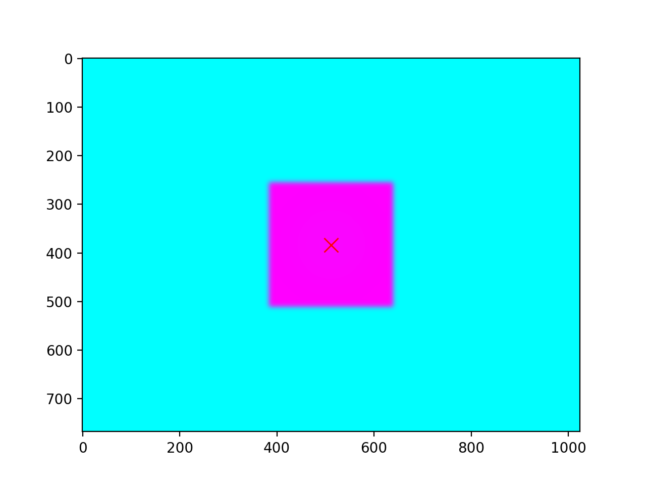
For example, let’s built a simple plugin that finds and plots an “X” at the center of the image:
from pylinac.core.image_generator import AS1000Image, FilteredFieldLayer, GaussianFilterLayer
from pylinac.core.image import DicomImage
from pylinac.core.metrics import MetricBase

class ImageCenterMetric(MetricBase):
    name = "Image Center"

    def calculate(self):
        return self.image.center

    def plot(self, axis: plt.Axes):
        axis.plot(self.image.center.x, self.image.center.y, 'rx', markersize=10)

# now we create an image to compute over
as1000 = AS1000Image(sid=1000)  # this will set the pixel size and shape automatically
as1000.add_layer(
    FilteredFieldLayer(field_size_mm=(100, 100))
)  # create a 100x100mm square field
as1000.add_layer(
    GaussianFilterLayer(sigma_mm=2)
)  # add an image-wide gaussian to simulate penumbra/scatter
ds = as1000.as_dicom()

# now we can compute the metric on the image
img = DicomImage.from_dataset(ds)
center = img.compute(metrics=ImageCenterMetric())
print(center)
img.plot()
(Source code, png, hires.png, pdf)
API#
- class pylinac.core.metrics.MetricBase[source]#
Base class for any 2D metric. This class is abstract and should not be instantiated.
The subclass should implement the
calculatemethod and thenameattribute.As a best practice, the
image_compatibilityattribute should be set to a list of image classes that the metric is compatible with. Image types that are not in the list will raise an error. This allows compatibility to be explicit. However, by default this is None and no compatibility checking is done.- context_calculate() Any[source]#
Calculate the metric, passing in an image copy so that modifications to the image don’t affect the original.
This is also kinda memory efficient since the original image is a reference. The copy here will get destroyed after the call returns vs keeping a copy around.
So at any given time, only 2x the memory is required instead of Nx. This is important when computing multiple metrics.
- class pylinac.core.metrics.DiskLocator(expected_position: Point | tuple[float, float], search_window: tuple[float, float], radius: float, radius_tolerance: float, detection_conditions: list[callable] = (<function is_round>, <function is_right_size_bb>, <function is_right_circumference>), name: str = 'Disk Region')[source]#
Calculates the weighted centroid of a disk/BB as a Point in an image where the disk is near an expected position and size.
- additional_plots() list[figure]#
Plot additional information on a separate figure as needed.
This should NOT show the figure. The figure will be shown via the
metric_plotsmethod. Calling show here would block other metrics from plotting their own separate metrics.
- context_calculate() Any#
Calculate the metric, passing in an image copy so that modifications to the image don’t affect the original.
This is also kinda memory efficient since the original image is a reference. The copy here will get destroyed after the call returns vs keeping a copy around.
So at any given time, only 2x the memory is required instead of Nx. This is important when computing multiple metrics.
- classmethod from_center(expected_position: Point | tuple[float, float], search_window: tuple[float, float], radius: float, radius_tolerance: float, detection_conditions: list[callable] = (<function is_round>, <function is_right_size_bb>, <function is_right_circumference>), name='Disk Region')#
Create a DiskRegion from a center point.
- classmethod from_center_physical(expected_position_mm: Point | tuple[float, float], search_window_mm: tuple[float, float], radius_mm: float, radius_tolerance_mm: float = 0.25, detection_conditions: list[callable] = (<function is_round>, <function is_right_size_bb>, <function is_right_circumference>), name='Disk Region')#
Create a DiskRegion using physical dimensions from the center point.
- classmethod from_physical(expected_position_mm: Point | tuple[float, float], search_window_mm: tuple[float, float], radius_mm: float, radius_tolerance_mm: float, detection_conditions: list[callable] = (<function is_round>, <function is_right_size_bb>, <function is_right_circumference>), name='Disk Region')#
Create a DiskRegion using physical dimensions.
- class pylinac.core.metrics.DiskRegion(expected_position: Point | tuple[float, float], search_window: tuple[float, float], radius: float, radius_tolerance: float, detection_conditions: list[callable] = (<function is_round>, <function is_right_size_bb>, <function is_right_circumference>), name: str = 'Disk Region')[source]#
A metric to find a disk/BB in an image where the BB is near an expected position and size. This will calculate the scikit-image regionprops of the BB.
- classmethod from_physical(expected_position_mm: Point | tuple[float, float], search_window_mm: tuple[float, float], radius_mm: float, radius_tolerance_mm: float, detection_conditions: list[callable] = (<function is_round>, <function is_right_size_bb>, <function is_right_circumference>), name='Disk Region')[source]#
Create a DiskRegion using physical dimensions.
- classmethod from_center(expected_position: Point | tuple[float, float], search_window: tuple[float, float], radius: float, radius_tolerance: float, detection_conditions: list[callable] = (<function is_round>, <function is_right_size_bb>, <function is_right_circumference>), name='Disk Region')[source]#
Create a DiskRegion from a center point.
- classmethod from_center_physical(expected_position_mm: Point | tuple[float, float], search_window_mm: tuple[float, float], radius_mm: float, radius_tolerance_mm: float = 0.25, detection_conditions: list[callable] = (<function is_round>, <function is_right_size_bb>, <function is_right_circumference>), name='Disk Region')[source]#
Create a DiskRegion using physical dimensions from the center point.
- calculate() RegionProperties[source]#
Find the scikit-image regiongprops of the BB.
This will apply a high-pass filter to the image iteratively. The filter starts at a very low percentile and increases until a region is found that meets the detection conditions.
- additional_plots() list[figure]#
Plot additional information on a separate figure as needed.
This should NOT show the figure. The figure will be shown via the
metric_plotsmethod. Calling show here would block other metrics from plotting their own separate metrics.
- context_calculate() Any#
Calculate the metric, passing in an image copy so that modifications to the image don’t affect the original.
This is also kinda memory efficient since the original image is a reference. The copy here will get destroyed after the call returns vs keeping a copy around.
So at any given time, only 2x the memory is required instead of Nx. This is important when computing multiple metrics.
- plot(axis: Axes) None#
Plot the metric