CatPhan¶

Overview¶

The CT module automatically analyzes DICOM images of a CatPhan 503, 504, 600, 604, 700, Quart DVT, or ACR phantoms acquired when doing CBCT or CT quality assurance. It can load a folder or zip file that the images are in and automatically correct for translational and rotational errors. It can analyze the HU regions and image scaling (CTP404), the high-contrast line pairs (CTP528) to calculate the modulation transfer function (MTF), the HU uniformity (CTP486), and Low Contrast (CTP515) on the corresponding slices.

For ACR and Quart phantoms, the equivalent sections are analyzed where applicable even though each module does not have an explicit name. Where intuitive similarities between the phantoms exist, the library usage is the same.

Features:

Automatic phantom registration - Your phantom can be tilted, rotated, or translated–pylinac will automatically register the phantom.
Automatic testing of all major modules - Major modules are automatically registered and analyzed.
Any scan protocol - Scan your CatPhan with any protocol; even scan it in a regular CT scanner. Any field size or field extent is allowed.

Running the Demo¶

To run one of the CatPhan demos, create a script or start an interpreter and input:

from pylinac import CatPhan504
cbct = CatPhan504.run_demo()  # the demo is a Varian high quality head scan

(Source code, png, hires.png, pdf)

Results will be also be printed to the console:

- CatPhan 504 QA Test -
HU Linearity ROIs: Air: -998.0, PMP: -200.0, LDPE: -102.0, Poly: -45.0, Acrylic: 115.0, Delrin: 340.0, Teflon: 997.0
HU Passed?: True
Low contrast visibility: 3.46
Geometric Line Average (mm): 49.95
Geometry Passed?: True
Measured Slice Thickness (mm): 2.499
Slice Thickness Passed? True
Uniformity ROIs: Top: 6.0, Right: -1.0, Bottom: 5.0, Left: 10.0, Center: 14.0
Uniformity index: -1.479
Integral non-uniformity: 0.0075
Uniformity Passed?: True
MTF 50% (lp/mm): 0.56
Low contrast ROIs "seen": 3

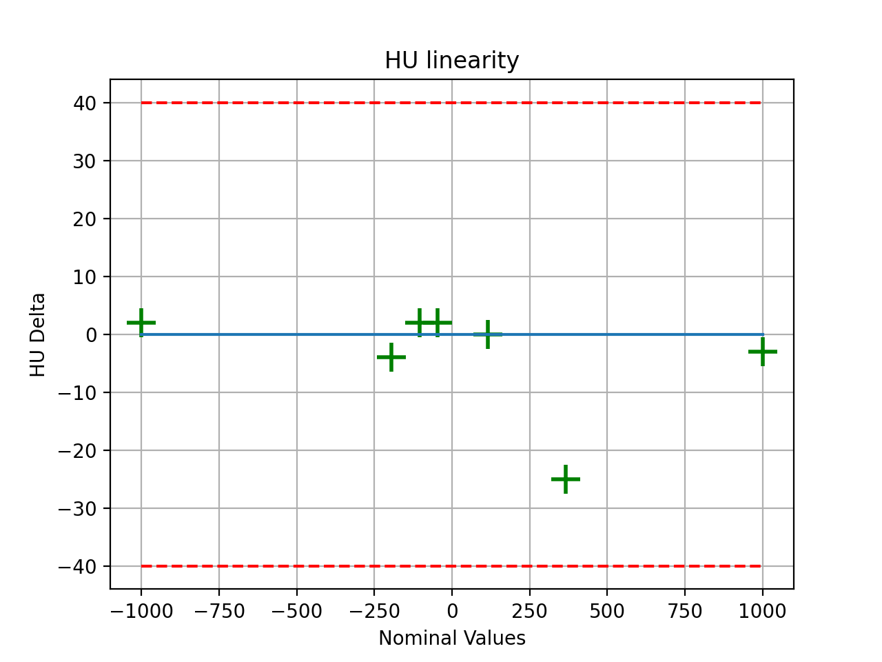
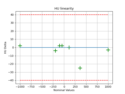
As well, you can plot and save individual pieces of the analysis such as linearity:

(Source code, png, hires.png, pdf)

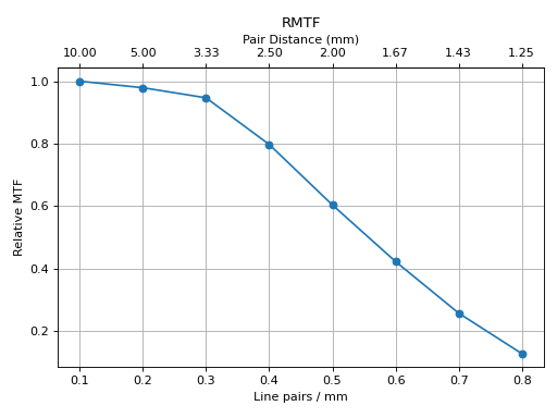
Or the rMTF:

cbct.plot_analyzed_subimage("rmtf")

(Source code, png, hires.png, pdf)

Or generate a PDF report:

cbct.publish_pdf("mycbct.pdf")

Image Acquisition¶

Acquiring a scan of a CatPhan has a few simple requirements:

The field of view must be larger than the phantom diameter + a few cm for clearance.
The phantom should not be touching any edge of the FOV.
The phantom shouldn’t touch the couch or other high-HU objects. This may cause localization issues finding the phantom. If the phantom doesn’t have an associated cradle, setting it on foam or something similar is recommended.
All modules must be visible.

Warning

This can cause strange results if not all modules are scanned. Furthermore, aligning axially to the white dots on the side of the catphan will not catch the inferior modules on a typical CBCT scan. We suggest aligning to the center of the HU module (the module inferior to the white dots) when acquiring via CBCT.

Typical Use¶

CatPhan analysis as done by this module closely follows what is specified in the CatPhan manuals, replacing the need for manual measurements. There are 4 CatPhan models that pylinac can analyze: CatPhan504, CatPhan503, & CatPhan600, & CatPhan604, each with their own class in pylinac. Let’s assume you have the CatPhan504 for this example. Using the other models/classes is exactly the same except the class name.

from pylinac import CatPhan504  # or import the CatPhan503 or CatPhan600

The minimum needed to get going is to:

Load images – Loading the DICOM images into your CatPhan object is done by passing the images in during construction. The most direct way is to pass in the directory where the images are:
```
cbct_folder = r"C:/QA Folder/CBCT/June monthly"
mycbct = CatPhan504(cbct_folder)
```
or load a zip file of the images:
```
zip_file = r"C:/QA Folder/CBCT/June monthly.zip"
mycbct = CatPhan504.from_zip(zip_file)
```
You can also use the demo images provided:
```
mycbct = CatPhan504.from_demo_images()
```
Analyze the images – Once the folder/images are loaded, tell pylinac to start analyzing the images. See the Algorithm section for details and analyze`() for analysis options:
```
mycbct.analyze()
```

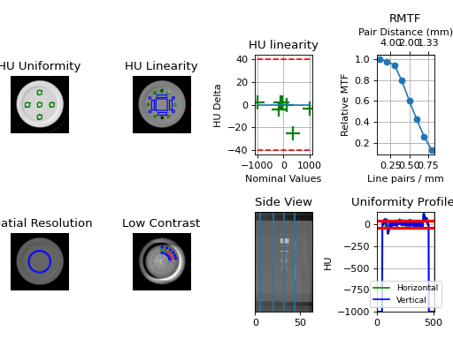
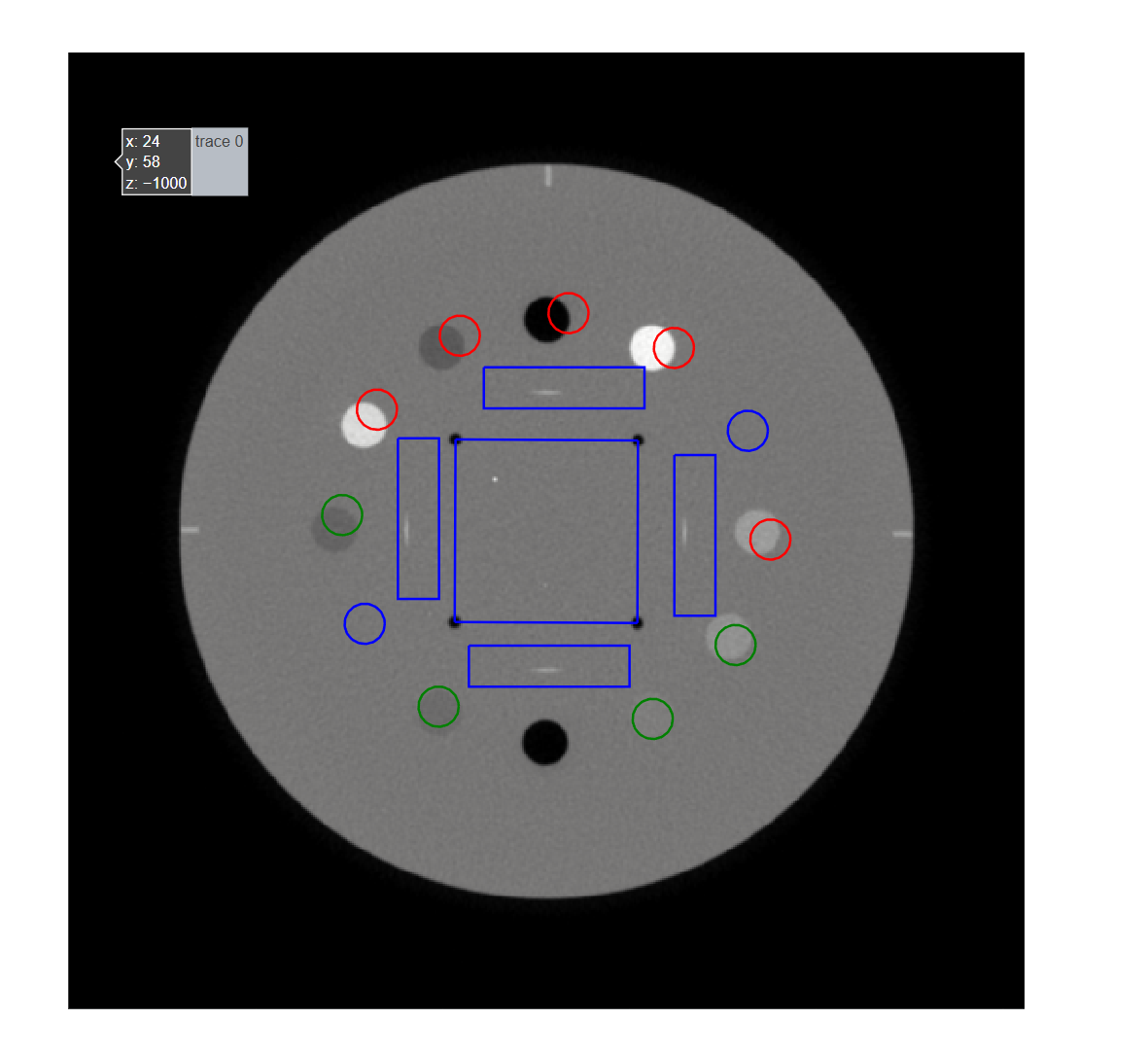
View the results – The CatPhan module can print out the summary of results to the console as well as draw a matplotlib image to show where the samples were taken and their values:

# print results to the console
print(mycbct.results())
# view analyzed images
mycbct.plot_analyzed_image()
# save the image
mycbct.save_analyzed_image("mycatphan504.png")
# generate PDF
mycbct.publish_pdf(
    "mycatphan.pdf", open_file=True
)  # open the PDF after saving as well.

Custom HU values¶

Added in version 3.16.

By default, expected HU values are drawn from the values stated in the manual. It’s possible to override one or more of the HU values of the CatPhan modules however. This is useful if you have a custom CatPhan or know the exact HU values of your phantom. To do so, pass in a dictionary of the HU values to the expected_hu_values parameter. The keys should be the name of the material and the values should be the HU value.

from pylinac import CatPhan504

# overrides the HU values of the Air and PMP regions
mycbct = CatPhan504(...)
mycbct.analyze(..., expected_hu_values={"Air": -999, "PMP": -203})
mycbct.plot_analyzed_image()

Note

Not all materials need to be overridden. Only the ones you want to override need to be passed in.

Keys¶

The keys to override for CatPhan504 and CatPhan503 are listed below along with the default value:

Air: -1000
PMP: -196
LDPE: -104
Poly: -47
Acrylic: 115
Delrin: 365
Teflon: 1000

The CatPhan600 has the above keys as well as:

Vial: 0

The CatPhan604 has the original keys as well as:

50% Bone: 725
20% Bone: 237

Slice Thickness¶

Added in version 3.12.

When measuring slice thickness in pylinac, slices are sometimes combined depending on the slice thickness. Scans with thin slices and low mAs can have very noisy wire ramp measurements. To compensate for this, pylinac will average over 3 slices (+/-1 from CTP404) if the slice thickness is <3.5mm. This will generally improve the statistics of the measurement. This is the only part of the algorithm that may use more than one slice.

If you’d like to override this, you can do so by setting the padding (aka straddle) explicitly. The straddle is the number of extra slices on each side of the HU module slice to use for slice thickness determination. The default is auto; set to an integer to explicitly use a certain amount of straddle slices. Typical values are 0, 1, and 2. So, a value of 1 averages over 3 slices, 2 => 5 slices, 3 => 7 slices, etc.

Note

This technique can be especially useful when your slices overlap.

from pylinac import CatPhan504  # applies to all catphans

ct = CatPhan504(...)
ct.analyze(..., thickness_slice_straddle=0)
...

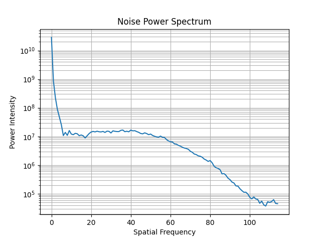
Noise Power Spectrum¶

Added in version 3.19.

The noise power spectrum (NPS) is a measure of the noise in the image using FFTs. It was added to comply with French regulations. It is calculated on the uniformity module (CTP486). Pylinac will provide the most populous frequency and the average power of the NPS.

from pylinac import CatPhan504

ct = CatPhan504(...)
ct.analyze(...)
ct.ctp486.avg_noise_power
ct.ctp486.max_noise_power_frequency
# plot the NPS
ct.ctp486.plot_noise_power_spectrum()

The resulting plot will look like so:

Advanced Use¶

Adjusting ROI locations¶

Added in version 3.29.

The ROIs of the Catphan modules can be individually adjusted (see Customizing module locations). However, sometimes the couch can get in the way or some other systematic shift of the ROIs occur. To globally adjust the ROIs use the parameters x_adjustment, y_adjustment, angle_adjustment, roi_size_factor, and scaling_factor in analyze. These parameters will shift the ROIs for all modules.

Note

This only applies to the x and y directions. To adjust where a specific module is or adjust the overall z-axis offset of the phantom you will need to perform the customization linked above.

from pylinac import CatPhan504

ct = CatPhan504(...)
ct.analyze(
    x_adjustment=5,
    y_adjustment=-2,
    angle_adjustment=3,
    roi_size_factor=1.1,
    scaling_factor=1,
)
ct.plot_analyzed_image()

Using `results_data`¶

Changed in version 3.0.

Using the catphan module in your own scripts? While the analysis results can be printed out, if you intend on using them elsewhere (e.g. in an API), they can be accessed the easiest by using the results_data() method which returns a CatPhanResult instance.

Note

While the pylinac tooling may change under the hood, this object should remain largely the same and/or expand. Thus, using this is more stable than accessing attrs directly.

Continuing from above:

data = mycbct.results_data()
data.catphan_model
data.ctp404.measured_slice_thickness_mm
# and more

# return as a dict
data_dict = mycbct.results_data(as_dict=True)
data_dict["ctp404"]["measured_slice_thickness_mm"]
...

Partial scans¶

While the default behavior of pylinac is to analyze all modules in the scan (in fact it will error out if they aren’t), the behavior can be customized. Pylinac always has to be aware of the CTP404 module as that’s the reference slice for everything else. Thus, if the 404 is not in the scan you’re SOL. However, if one of the other modules is not present you can remove or adjust its offset by subclassing and overloading the modules attr:

from pylinac import CatPhan504  # works for any of the other phantoms too
from pylinac.ct import CTP515, CTP486


class PartialCatPhan504(CatPhan504):
    modules = {
        CTP486: {"offset": -65},
        CTP515: {"offset": -30},
        # the CTP528 was omitted
    }


ct = PartialCatPhan504.from_zip(...)  # use like normal

Examining rMTF¶

The rMTF can be calculated ad hoc like so. Note that CTP528 must be present (see above):

ct = ...  # load a dataset like normal
ct.analyze()
ct.ctp528.mtf.relative_resolution(x=40)  # get the rMTF (lp/mm) at 40% resolution

Localization Variance¶

There are some instances where the HU of the phantom density modules are drastically different than the expected values. This most often occurs with Elekta linacs and Siemens DirectDensity reconstruction. This will usually result in one of two errors: No slices were found that resembled the HU linearity module or The physical scan extent does not match the module configuration....

To work around this, note the values of the air bubble, teflon HU insert, and the mean HU value of the phantom slice (anywhere that’s not an HU insert or hole). Set the hu_origin_slice_variance class attribute to the lower of the difference between the air and phantom mean and the teflon and phantom mean.

If, e.g., the air is -1000, the mean value of the phantom is 33, and the Teflon is 350 set the variance to be <= 317 (350-33). The default is 400. If the HU values are near their correct value you shouldn’t have to do this.

from pylinac import CatPhan504

ct = CatPhan504.from_zip(...)
ct.hu_origin_slice_variance = 275
ct.analyze()

In RadMachine, the “HU localization variance” parameter can be used to fix this. See Analysis Parameters.

Customizing module locations¶

Similar to partial scans, to modify the module location(s), overload the modules attr and edit the offset value. The value is in mm:

from pylinac import CatPhan504  # works for any of the other phantoms too
from pylinac.ct import CTP515, CTP486, CTP528


# create custom catphan with module locations
class OffsetCatPhan504(CatPhan504):
    modules = {
        CTP486: {"offset": -60},  # normally -65
        CTP528: {"offset": 30},
        CTP515: {"offset": -25},  # normally -30
    }


ct = OffsetCatPhan504.from_zip(...)  # use like normal

Customizing Modules¶

You can also customize modules themselves in v2.4+. Customization should always be done by subclassing an existing module and overloading the attributes. Then, pass in the new custom module into the parent CatPhan class. The easiest way to get started is copy the relevant attributes from the existing code.

As an example, let’s override the angles of the ROIs for CTP404.

from pylinac.ct import CatPhan504, CTP404CP504


# first, customize the module
class CustomCTP404(CTP404CP504):
    roi_dist_mm = 58.7  # this is the default value; we repeat here because it's easy to copy from source
    roi_radius_mm = 5  # ditto
    roi_settings = {
        "Air": {
            "value": -1000,
            "angle": -93,  # changed 'angle' from -90 to -93
            "distance": roi_dist_mm,
            "radius": roi_radius_mm,
        },
        "PMP": {
            "value": -196,
            "angle": -122,  # changed 'angle' from -120 to -122
            "distance": roi_dist_mm,
            "radius": roi_radius_mm,
        },
        # add other ROIs as appropriate
    }


# then, pass to the CatPhan model
class CustomCP504(CatPhan504):
    modules = {
        CustomCTP404: {"offset": 0}
        # add other modules here as appropriate
    }


# use like normal
ct = CustomCP504(...)

Warning

If you overload the roi_settings or modules attributes, you are responsible for filling it out completely. I.e. when you overload it’s not partial. In the above example if you want other CTP modules you must populate them.

Analysis Parameters¶

This applies to the 503, 504, 600, and 604. Model-specific parameters are called out.

pylinac

See analyze() for details.

RadMachine

HU Tolerance: The tolerance for the HU linearity of the inserts.
Scaling Tolerance: The tolerance for the scaling of the phantom in mm. Uses the geometric nodes of the CTP404 module.
Slice Thickness tolerance: The tolerance for the slice thickness in mm. Uses the ramped wire.
Slice thickness straddle: The number of slices to combine when measuring slice thickness.If blank, will combine thin slices automatically. Combining slices gives a more robust evaluation of the measurement in noisy/thin-slice images.
Minimum low contrast ROIs: The minimum number of low contrast ROIs that must be “seen” to pass.
Air HU: The reference HU value of the air ROI.
PMP HU: The reference HU value of the PMP ROI.
LDPE HU: The reference HU value of the LDPE ROI.
Poly HU: The reference HU value of the Polystyrene ROI.
Acrylic HU: The reference HU value of the Acrylic ROI.
Delrin HU: The reference HU value of the Delrin ROI.
Teflon HU: The reference HU value of the Teflon ROI.
Water Vial: The reference HU value of the water vial ROI.

Note

Only applicable for the CatPhan 600
Bone 20%: The reference HU value of the 20% bone ROI.

Note

Only applicable for the CatPhan 604
Bone 50%: The reference HU value of the 50% bone ROI.

Note

Only applicable for the CatPhan 604
Contrast definition: The method used to calculate the contrast of the low contrast ROIs. See Contrast.
Low contrast detection threshold: The threshold used to determine if a low contrast ROI was “seen”. See Visibility.
HU localization variance: The minimum difference between the phantom mean and the air or Teflon HU values. Used for localization only. See Localization Variance.
X adjustment: A fine-tuning adjustment to the detected x-coordinate of the phantom center. This will move the detected phantom position by this amount in the x-direction in mm. Positive values move the phantom to the right.
Y adjustment: A fine-tuning adjustment to the detected y-coordinate of the phantom center. This will move the detected phantom position by this amount in the y-direction in mm. Positive values move the phantom down.
Angle adjustment: A fine-tuning adjustment to the detected angle of the phantom. This will rotate the phantom by this amount in degrees. Positive values rotate the phantom clockwise.
ROI size factor: A fine-tuning adjustment to the ROI sizes of the phantom. This will scale the ROIs by this amount. Positive values increase the ROI sizes. In contrast to the scaling adjustment, this adjustment effectively makes the ROIs bigger or smaller, but does not adjust their position.
Scaling factor: A fine-tuning adjustment to the detected magnification of the phantom. This will zoom the ROIs and phantom outline (if applicable) by this amount. In contrast to the roi size adjustment, the scaling adjustment effectively moves the phantom and ROIs closer or further from the phantom center. I.e. this zooms the outline and ROI positions, but not ROI size.
Origin slice: The slice number that corresponds to the HU linearity slice. This is a fallback mechanism in case the automatic detection fails.

Algorithm¶

The CatPhan module is based on the tests and values given in the respective CatPhan manual. The algorithm works like such:

Allowances¶

The images can be any size.
The phantom can have significant translation in all 3 directions.
The phantom can have significant roll and moderate yaw and pitch.

Restrictions¶

Warning

Analysis can fail or give unreliable results if any Restriction is violated.

All of the modules defined in the modules attribute must be within the scan extent.
Scan slices are not expected to overlap.

Warning

Overlapping slices are not generally a problem other than the slice thickness measurement. See the Slice Thickness section for how to override this to get a valid slice thickness in such a situation.
The HU values of the linearity inserts are within ~30% of their expected values. See Localization Variance for how to override this. if using an Elekta machine or special reconstruction algorithm.

Pre-Analysis¶

Determine image properties – Upon load, the image set is analyzed for its DICOM properties to determine mm/pixel spacing, rescale intercept and slope, manufacturer, etc.
Convert to HU – The entire image set is converted from its raw values to HU by applying the rescale intercept and slope which is contained in the DICOM properties.
Find the phantom z-location – Upon loading, all the images are scanned to determine where the HU linearity module (CTP404) is located. This is accomplished by examining each image slice and looking for 2 things:
- If the CatPhan is in the image. At the edges of the scan this may not be true.
- If a circular profile has characteristics like the CTP404 module. If the CatPhan is in the image, a circular profile is taken at the location where the HU linearity regions of interest are located. If the profile contains low, high, and lots of medium values then it is very likely the HU linearity module. All such slices are found and the median slice is set as the HU linearity module location. All other modules are located relative to this position.

Analysis¶

Determine phantom roll – Precise knowledge of the ROIs to analyze is important, and small changes in rotation could invalidate automatic results. The roll of the phantom is determined by examining the HU module and converting to a binary image. The air holes are then located and the angle of the two holes determines the phantom roll.

Note

For each step below, the “module” analyzed is actually the mean, median, or maximum of 3 slices (+/-1 slice around and including the nominal slice) to ensure robust measurements. Also, for each step/phantom module, the phantom center is determined, which corrects for the phantom pitch and yaw.

Additionally, values tend to be lazy (computed only when asked for), thus the calculations listed may sometimes be performed only when asked for.

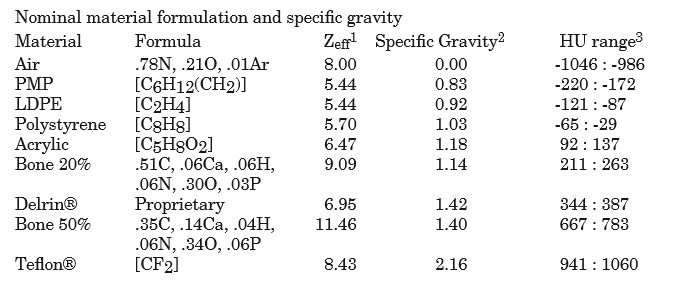
Determine HU linearity – The HU module (CTP404) contains several materials with different HU values. Using hardcoded angles (corrected for roll) and radius from the center of the phantom, circular ROIs are sampled which correspond to the HU material regions. The median pixel value of the ROI is the stated HU value. Nominal HU values are taken as the mean of the range given in the manual(s):

Note

As of v3.16, these can be overridden: Custom HU values.
Determine HU uniformity – HU uniformity (CTP486) is calculated in a similar manner to HU linearity, but within the CTP486 module/slice.
Calculate Geometry/Scaling – The HU module (CTP404), besides HU materials, also contains several “nodes” which have an accurate spacing (50 mm apart). Again, using hardcoded but corrected angles, the area around the 4 nodes are sampled and then a threshold is applied which identifies the node within the ROI sample. The center of mass of the node is determined and then the space between nodes is calculated.
Calculate Spatial Resolution/MTF – The Spatial Resolution module (CTP528) contains 21 pairs of aluminum bars having varying thickness, which also corresponds to the thickness between the bars. One unique advantage of these bars is that they are all focused on and equally distant to the phantom center. This is taken advantage of by extracting a CollapsedCircleProfile about the line pairs. The peaks and valleys of the profile are located; peaks and valleys of each line pair are used to calculated the MTF. The relative MTF (i.e. normalized to the first line pair) is then calculated from these values. See Modulation Transfer Function.
Calculate Low Contrast Resolution – Low contrast is inherently difficult to determine since detectability of humans is not simply contrast based. Pylinac’s analysis uses both the contrast value of the ROI as well as the ROI size to compute a “detectability” score. ROIs above the score are said to be “seen”, while those below are not seen. Only the 1.0% supra-slice ROIs are examined. Two background ROIs are sampled on either side of the ROI contrast set. See Visibility for equation details.
Calculate Slice Thickness – Slice thickness is measured by determining the FWHM of the wire ramps in the CTP404 module. A profile of the area around each wire ramp is taken, and the FWHM is determined from the profile. The profiles are averaged and the value is converted from pixels to mm and multiplied by 0.42 (Catphan manual “Scan Slice Geometry” section). Also see Slice Thickness.

Post-Analysis¶

Test if values are within tolerance – For each module, the determined values are compared with the nominal values. If the difference between the two is below the specified tolerance then the module passes.

Interpreting Results¶

The results of a CatPhan analysis in RadMachine or from results_data are:

catphan_model: The model of CatPhan that was analyzed.
catphan_roll_deg: The roll of the phantom in degrees.
origin_slice: The “origin” slice number. For CatPhan, this is the center of the HU module.
num_images: The number of images in the passed dataset.
ctp404: The results of the CTP404 module (HU linearity, spacing) with the following items:
- offset: The offset of the module from the origin slice in mm.
- low_contrast_visibility: The low contrast visibility score.
- thickness_passed: Whether the slice thickness passed.
- measured_slice_thickness_mm: The measured slice thickness in mm.
- thickness_num_slices_combined: The number of slices combined when measuring slice thickness.
- geometry_passed: Whether the geometry test passed, using the 4 nodes.
- avg_line_distance_mm: The average distance between the 4 nodes in mm.
- line_distances_mm: A list of the individual distances between nodes.
- hu_linearity_passed: Whether all the HU ROIs were within tolerance.
- hu_tolerance: The tolerance used for the HU linearity test.
- hu_rois: A dictionary of the HU ROIs and their values. The keys will be the material name such as Acrylic. The values for each ROI will be a dictionary with the following keys:
  - name: The name of the material.
  - value: The measured HU value.
  - nominal_value: The nominal HU value.
  - passed: Whether the ROI passed.
  - stdev: The pixel value standard deviation of the ROI.
  - difference: The difference between the measured and nominal values.
ctp486: The results of the CTP486 module (HU uniformity) with the following items:
- uniformity_index: The uniformity index as defined in Equation 2 of Elstrom et al.
- integral_non_uniformity: The integral non-uniformity as defined in Equation 1 of Elstrom et al.
- nps_avg_power: The average power of the noise power spectrum. See Noise Power.
- nps_max_freq: The most populous frequency of the noise power spectrum.
- passed: Whether the uniformity test passed.
- rois: A dictionary of the uniformity ROIs and their values. The keys will be the region name such as Top. The values for each ROI will be a dictionary with the following keys:
  - name: The region the ROI was sampled from.
  - value: The measured HU value.
  - nominal_value: The nominal HU value.
  - passed: Whether the ROI passed.
  - stdev: The pixel value standard deviation of the ROI.
  - difference: The difference between the measured and nominal values.
ctp528: The results of the CTP528 (spatial resolution) module with the following items:
- start_angle_radians: The angle where the circular profile started.
- mtf_lp_mm: A dictionary from 10% to 90% resolution in steps of 10 of the MTF in lp/mm. E.g. '20': 0.748. To get the MTF at a specific resolution see Examining rMTF.
- roi_settings: A dictionary of the settings used for each MTF ROI. The key names are region_<n> where <n> is the region number. The values are a dictionary with the following keys:
  - start: The start angle of the ROI in degrees relative to the start_angle_radians setting.
  - end: The end angle of the ROI in degrees relative to the start_angle_radians setting.
  - num peaks: The number of peaks found in the profile.
  - num valleys: The number of valleys found in the profile.
  - peak spacing: The spacing between peaks in pixels.
  - gap size (cm): The size of the gap between the bars in cm.
  - lp/mm: The number of line pairs per mm.
ctp515: The results of the CTP515 (Low contrast) module with the following items:
- cnr_threshold: The contrast-to-noise ratio threshold used to determine if a low contrast ROI was “seen”.
- num_rois_seen: The number of ROIs that were above the threshold; ie. “seen”.
- roi_settings: The settings used for each low contrast ROI. The key names are n where <n> is the size of the ROI. The values are a dictionary with the following keys:
  - angle: The angle of the ROI in degrees.
  - distance: The distance from the phantom center in mm.
  - radius: The radius of the ROI in mm.
  - distance_pixels: The distance from the phantom center in pixels.
  - angle_corrected: The angle of the ROI corrected for phantom roll.
  - radius_pixels: The radius of the ROI in pixels.
- roi_results: Results of the low contrast ROIs and their values. The keys will be the size of the ROI such as '9'. The values for each ROI will be a dictionary with the following keys:
  - contrast method: The method used to calculate the contrast. See Contrast.
  - visibility: The visibility score of the ROI.
  - visibility threshold: The threshold used to determine if the ROI was “seen”.
  - passed visibility: Whether the ROI was “seen”.
  - contrast: The contrast of the ROI.
  - cnr: The contrast-to-noise ratio of the ROI.
  - signal to noise: The signal-to-noise ratio of the ROI.

Troubleshooting¶

First, check the general Troubleshooting section. Most problems in this module revolve around getting the data loaded.

If you’re having trouble getting your dataset in, make sure you’re loading the whole dataset. Also make sure you’ve scanned the whole phantom.
Make sure there are no external markers on the CatPhan (e.g. BBs), otherwise the localization algorithm will not be able to properly locate the phantom within the image.
Ensure that the FOV is large enough to encompass the entire phantom. If the scan is cutting off the phantom in any way it will not identify it.
The phantom should never touch the edge of an image, see above point.
Make sure you’re loading the right CatPhan class. I.e. using a CatPhan600 class on a CatPhan504 scan may result in errors or erroneous results.

Siemens DirectDensity¶

If you are using a Siemens scanner with DirectDensity, the HU values of the phantom may be incorrect. This is because the algorithm is not designed for man-made materials. See the white paper here, specifically page 13, “Compatibility and limitations”.

Usually, scans from this type of reconstruction drastically underestimate the HU of Teflon. This most often causes a failure to find the HU linearity module. See Localization Variance for how to correct this.

API Documentation¶

Main classes¶

These are the classes a typical user may interface with.

class pylinac.ct.CatPhan504(folderpath: str | Sequence[str] | Path | Sequence[Path] | Sequence[BytesIO], check_uid: bool = True, memory_efficient_mode: bool = False, is_zip: bool = False)[source]¶

Bases: CatPhanBase

A class for loading and analyzing CT DICOM files of a CatPhan 504. Can be from a CBCT or CT scanner Analyzes: Uniformity (CTP486), High-Contrast Spatial Resolution (CTP528), Image Scaling & HU Linearity (CTP404), and Low contrast (CTP515).

Parameters¶

folderpathstr, list of strings, or Path to folder: String that points to the CBCT image folder location.
check_uidbool: Whether to enforce raising an error if more than one UID is found in the dataset.
memory_efficient_modebool: Whether to use a memory efficient mode. If True, the DICOM stack will be loaded on demand rather than all at once. This will reduce the memory footprint but will be slower by ~25%. Default is False.

Raises¶

NotADirectoryError: If folder str passed is not a valid directory.
FileNotFoundError: If no CT images are found in the folder

static run_demo(show: bool = True)[source]¶: Run the CBCT demo using high-quality head protocol images.

analyze(hu_tolerance: int | float = 40, scaling_tolerance: int | float = 1, thickness_tolerance: int | float = 0.2, low_contrast_tolerance: int | float = 1, cnr_threshold: int | float = 15, zip_after: bool = False, contrast_method: str = 'Michelson', visibility_threshold: float = 0.15, thickness_slice_straddle: str | int = 'auto', expected_hu_values: dict[str, int | float] | None = None, x_adjustment: float = 0, y_adjustment: float = 0, angle_adjustment: float = 0, roi_size_factor: float = 1, scaling_factor: float = 1, origin_slice: int | None = None)¶

Single-method full analysis of CBCT DICOM files.

Parameters¶

hu_toleranceint: The HU tolerance value for both HU uniformity and linearity.
scaling_tolerancefloat, int: The scaling tolerance in mm of the geometric nodes on the HU linearity slice (CTP404 module).
thickness_tolerancefloat, int: The tolerance of the thickness calculation in mm, based on the wire ramps in the CTP404 module.

Warning

Thickness accuracy degrades with image noise; i.e. low mAs images are less accurate.
low_contrast_toleranceint: The number of low-contrast bubbles needed to be “seen” to pass.
cnr_thresholdfloat, int: The threshold for “detecting” low-contrast image. See RTD for calculation info.

Deprecated since version 3.0: Use visibility parameter instead.
zip_afterbool: If the CT images were not compressed before analysis and this is set to true, pylinac will compress the analyzed images into a ZIP archive.
contrast_method: The contrast equation to use. See Low contrast.
visibility_threshold: The threshold for detecting low-contrast ROIs. Use instead of cnr_threshold. Follows the Rose equation. See Visibility.
thickness_slice_straddle: The number of extra slices on each side of the HU module slice to use for slice thickness determination. The rationale is that for thin slices the ramp FWHM can be very noisy. I.e. a 1mm slice might have a 100% variation with a low-mAs protocol. To account for this, slice thicknesses < 3.5mm have 1 slice added on either side of the HU module (so 3 total slices) and then averaged. The default is ‘auto’, which follows the above logic. Set to an integer to explicitly use a certain amount of padding. Typical values are 0, 1, and 2.

Warning

This is the padding on either side. So a value of 1 => 3 slices, 2 => 5 slices, 3 => 7 slices, etc.
expected_hu_values: An optional dictionary of the expected HU values for the HU linearity module. The keys are the ROI names and the values are the expected HU values. If a key is not present or the parameter is None, the default values will be used.
x_adjustment: float: A fine-tuning adjustment to the detected x-coordinate of the phantom center. This will move the detected phantom position by this amount in the x-direction in mm. Positive values move the phantom to the right.
y_adjustment: float: A fine-tuning adjustment to the detected y-coordinate of the phantom center. This will move the detected phantom position by this amount in the y-direction in mm. Positive values move the phantom down.
angle_adjustment: float: A fine-tuning adjustment to the detected angle of the phantom. This will rotate the phantom by this amount in degrees. Positive values rotate the phantom clockwise.
roi_size_factor: float: A fine-tuning adjustment to the ROI sizes of the phantom. This will scale the ROIs by this amount. Positive values increase the ROI sizes. In contrast to the scaling adjustment, this adjustment effectively makes the ROIs bigger or smaller, but does not adjust their position.
scaling_factor: float: A fine-tuning adjustment to the detected magnification of the phantom. This will zoom the ROIs and phantom outline (if applicable) by this amount. In contrast to the roi size adjustment, the scaling adjustment effectively moves the phantom and ROIs closer or further from the phantom center. I.e. this zooms the outline and ROI positions, but not ROI size.
origin_sliceint, None: The slice number of the HU linearity module. If None, the slice will be determined automatically. This is a fallback method if the automatic localization algorithm fails.

property catphan_size: float¶: The expected size of the phantom in pixels, based on a 20cm wide phantom.

clear_captured_warnings() → None¶: Clear the list of captured warnings.

find_origin_slice() → int¶

Using a brute force search of the images, find the median HU linearity slice.

This method walks through all the images and takes a collapsed circle profile where the HU linearity ROIs are. If the profile contains both low (<800) and high (>800) HU values and most values are the same (i.e. it’s not an artifact), then it can be assumed it is an HU linearity slice. The median of all applicable slices is the center of the HU slice.

Returns¶

int: The middle slice of the HU linearity module.

find_phantom_axis()¶

We fit all the center locations of the phantom across all slices to a 1D poly function instead of finding them individually for robustness.

Normally, each slice would be evaluated individually, but the RadMachine jig gets in the way of detecting the HU module (🤦‍♂️). To work around that in a backwards-compatible way we instead look at all the slices and if the phantom was detected, capture the phantom center. ALL the centers are then fitted to a 1D poly function and passed to the individual slices. This way, even if one slice is messed up (such as because of the phantom jig), the poly function is robust to give the real center based on all the other properly-located positions on the other slices.

find_phantom_roll(func: Callable | None = None) → float¶

Determine the “roll” of the phantom.

This algorithm uses the two air bubbles in the HU slice and the resulting angle between them.

Parameters¶

func: A callable to sort the air ROIs.

Returns¶

float : the angle of the phantom in degrees.

classmethod from_demo_images()¶: Construct a CBCT object from the demo images.

classmethod from_url(url: str, check_uid: bool = True)¶

Instantiate a CBCT object from a URL pointing to a .zip object.

Parameters¶

urlstr: URL pointing to a zip archive of CBCT images.
check_uidbool: Whether to enforce raising an error if more than one UID is found in the dataset.

classmethod from_zip(zip_file: str | ZipFile | BinaryIO, check_uid: bool = True, memory_efficient_mode: bool = False)¶

Construct a CBCT object and pass the zip file.

Parameters¶

zip_filestr, ZipFile: Path to the zip file or a ZipFile object.
check_uidbool: Whether to enforce raising an error if more than one UID is found in the dataset.
memory_efficient_modebool: Whether to use a memory efficient mode. If True, the DICOM stack will be loaded on demand rather than all at once. This will reduce the memory footprint but will be slower by ~25%. Default is False.

Raises¶

FileExistsError : If zip_file passed was not a legitimate zip file. FileNotFoundError : If no CT images are found in the folder

get_captured_warnings() → list[dict]¶: Retrieve the list of captured warnings.

localize(origin_slice: int | None) → None¶: Find the slice number of the catphan’s HU linearity module and roll angle

property mm_per_pixel: float¶: The millimeters per pixel of the DICOM images.

property num_images: int¶: The number of images loaded.

plot_analyzed_image(show: bool = True, **plt_kwargs) → None¶

Plot the images used in the calculation and summary data.

Parameters¶

showbool: Whether to plot the image or not.
plt_kwargsdict: Keyword args passed to the plt.figure() method. Allows one to set things like figure size.

plot_analyzed_subimage(subimage: str = 'hu', delta: bool = True, show: bool = True) → Figure | None¶

Plot a specific component of the CBCT analysis.

Parameters¶

subimage{‘hu’, ‘un’, ‘sp’, ‘lc’, ‘mtf’, ‘lin’, ‘prof’, ‘side’}

The subcomponent to plot. Values must contain one of the following letter combinations. E.g. linearity, linear, and lin will all draw the HU linearity values.

hu draws the HU linearity image.
un draws the HU uniformity image.
sp draws the Spatial Resolution image.
lc draws the Low Contrast image (if applicable).
mtf draws the RMTF plot.
lin draws the HU linearity values. Used with delta.
prof draws the HU uniformity profiles.
side draws the side view of the phantom with lines of the module locations.

deltabool

Only for use with lin. Whether to plot the HU delta or actual values.

showbool

Whether to actually show the plot.

plot_side_view(axis: Axes) → None¶: Plot a view of the scan from the side with lines showing detected module positions

plotly_analyzed_images(show: bool = True, show_colorbar: bool = True, show_legend: bool = True, **kwargs) → dict[str, Figure]¶

Plot the analyzed set of images to Plotly figures.

Parameters¶

showbool: Whether to show the plot.
show_colorbarbool: Whether to show the colorbar on the plot.
show_legendbool: Whether to show the legend on the plot.
kwargs: Additional keyword arguments to pass to the plot.

Returns¶

dict: A dictionary of the Plotly figures where the key is the name of the image and the value is the figure.

Publish (print) a PDF containing the analysis and quantitative results.

Parameters¶

filename(str, file-like object}: The file to write the results to.
notesstr, list of strings: Text; if str, prints single line. If list of strings, each list item is printed on its own line.
open_filebool: Whether to open the file using the default program after creation.
metadatadict: Extra data to be passed and shown in the PDF. The key and value will be shown with a colon. E.g. passing {‘Author’: ‘James’, ‘Unit’: ‘TrueBeam’} would result in text in the PDF like: ————– Author: James Unit: TrueBeam ————–
logo: Path, str: A custom logo to use in the PDF report. If nothing is passed, the default pylinac logo is used.

refine_origin_slice(initial_slice_num: int) → int¶: Apply a refinement to the origin slice. This was added to handle the catphan 604 at least due to variations in the length of the HU plugs.

results(as_list: bool = False) → str | list[list[str]]¶

Return the results of the analysis as a string. Use with print().

Parameters¶

as_listbool: Whether to return as a list of list of strings vs single string. Pretty much for internal usage.

results_data(as_dict: bool = False, as_json: bool = False, by_alias: bool = False, exclude: set[str] | None = None) → T | dict | str¶

Present the results data and metadata as a dataclass, dict, or tuple. The default return type is a dataclass.

Parameters¶

as_dictbool: If True, return the results as a dictionary.
as_jsonbool: If True, return the results as a JSON string. Cannot be True if as_dict is True.
by_aliasbool: If True, use the alias names of the dataclass fields. These are generally the more human-readable names.
excludeset: A set of fields to exclude from the results data.

save_analyzed_image(filename: str | Path | BinaryIO, **kwargs) → None¶

Save the analyzed summary plot.

Parameters¶

filenamestr, file object: The name of the file to save the image to.
kwargs :: Any valid matplotlib kwargs.

save_analyzed_subimage(filename: str | BinaryIO, subimage: str = 'hu', delta: bool = True, **kwargs) → Figure | None¶

Save a component image to file.

Parameters¶

filenamestr, file object: The file to write the image to.
subimagestr: See plot_analyzed_subimage() for parameter info.
deltabool: Only for use with lin. Whether to plot the HU delta or actual values.

to_quaac(path: str | Path, performer: User, primary_equipment: Equipment, format: Literal['json', 'yaml'] = 'yaml', attachments: list[Attachment] | None = None, overwrite: bool = False, **kwargs) → None¶

Write an analysis to a QuAAC file. This will include the items from results_data() and the PDF report.

Parameters¶

pathstr, Path: The file to write the results to.
performerUser: The user who performed the analysis.
primary_equipmentEquipment: The equipment used in the analysis.
format{‘json’, ‘yaml’}: The format to write the file in.
attachmentslist of Attachment: Additional attachments to include in the QuAAC file.
overwritebool: Whether to overwrite the file if it already exists.
kwargs: Additional keyword arguments to pass to the Document instantiation.

class pylinac.ct.CatPhan503(folderpath: str | Sequence[str] | Path | Sequence[Path] | Sequence[BytesIO], check_uid: bool = True, memory_efficient_mode: bool = False, is_zip: bool = False)[source]¶

Bases: CatPhanBase

A class for loading and analyzing CT DICOM files of a CatPhan 503. Analyzes: Uniformity (CTP486), High-Contrast Spatial Resolution (CTP528), Image Scaling & HU Linearity (CTP404).

Parameters¶

folderpathstr, list of strings, or Path to folder: String that points to the CBCT image folder location.
check_uidbool: Whether to enforce raising an error if more than one UID is found in the dataset.
memory_efficient_modebool: Whether to use a memory efficient mode. If True, the DICOM stack will be loaded on demand rather than all at once. This will reduce the memory footprint but will be slower by ~25%. Default is False.

Raises¶

NotADirectoryError: If folder str passed is not a valid directory.
FileNotFoundError: If no CT images are found in the folder

static run_demo(show: bool = True)[source]¶: Run the CBCT demo using high-quality head protocol images.

Single-method full analysis of CBCT DICOM files.

Parameters¶

hu_toleranceint: The HU tolerance value for both HU uniformity and linearity.
scaling_tolerancefloat, int: The scaling tolerance in mm of the geometric nodes on the HU linearity slice (CTP404 module).
thickness_tolerancefloat, int: The tolerance of the thickness calculation in mm, based on the wire ramps in the CTP404 module.

Warning

Thickness accuracy degrades with image noise; i.e. low mAs images are less accurate.
low_contrast_toleranceint: The number of low-contrast bubbles needed to be “seen” to pass.
cnr_thresholdfloat, int: The threshold for “detecting” low-contrast image. See RTD for calculation info.

Deprecated since version 3.0: Use visibility parameter instead.
zip_afterbool: If the CT images were not compressed before analysis and this is set to true, pylinac will compress the analyzed images into a ZIP archive.
contrast_method: The contrast equation to use. See Low contrast.
visibility_threshold: The threshold for detecting low-contrast ROIs. Use instead of cnr_threshold. Follows the Rose equation. See Visibility.
thickness_slice_straddle: The number of extra slices on each side of the HU module slice to use for slice thickness determination. The rationale is that for thin slices the ramp FWHM can be very noisy. I.e. a 1mm slice might have a 100% variation with a low-mAs protocol. To account for this, slice thicknesses < 3.5mm have 1 slice added on either side of the HU module (so 3 total slices) and then averaged. The default is ‘auto’, which follows the above logic. Set to an integer to explicitly use a certain amount of padding. Typical values are 0, 1, and 2.

Warning

This is the padding on either side. So a value of 1 => 3 slices, 2 => 5 slices, 3 => 7 slices, etc.
expected_hu_values: An optional dictionary of the expected HU values for the HU linearity module. The keys are the ROI names and the values are the expected HU values. If a key is not present or the parameter is None, the default values will be used.
x_adjustment: float: A fine-tuning adjustment to the detected x-coordinate of the phantom center. This will move the detected phantom position by this amount in the x-direction in mm. Positive values move the phantom to the right.
y_adjustment: float: A fine-tuning adjustment to the detected y-coordinate of the phantom center. This will move the detected phantom position by this amount in the y-direction in mm. Positive values move the phantom down.
angle_adjustment: float: A fine-tuning adjustment to the detected angle of the phantom. This will rotate the phantom by this amount in degrees. Positive values rotate the phantom clockwise.
roi_size_factor: float: A fine-tuning adjustment to the ROI sizes of the phantom. This will scale the ROIs by this amount. Positive values increase the ROI sizes. In contrast to the scaling adjustment, this adjustment effectively makes the ROIs bigger or smaller, but does not adjust their position.
scaling_factor: float: A fine-tuning adjustment to the detected magnification of the phantom. This will zoom the ROIs and phantom outline (if applicable) by this amount. In contrast to the roi size adjustment, the scaling adjustment effectively moves the phantom and ROIs closer or further from the phantom center. I.e. this zooms the outline and ROI positions, but not ROI size.
origin_sliceint, None: The slice number of the HU linearity module. If None, the slice will be determined automatically. This is a fallback method if the automatic localization algorithm fails.

property catphan_size: float¶: The expected size of the phantom in pixels, based on a 20cm wide phantom.

clear_captured_warnings() → None¶: Clear the list of captured warnings.

find_origin_slice() → int¶

Using a brute force search of the images, find the median HU linearity slice.

Returns¶

int: The middle slice of the HU linearity module.

find_phantom_axis()¶

We fit all the center locations of the phantom across all slices to a 1D poly function instead of finding them individually for robustness.

find_phantom_roll(func: Callable | None = None) → float¶

Determine the “roll” of the phantom.

This algorithm uses the two air bubbles in the HU slice and the resulting angle between them.

Parameters¶

func: A callable to sort the air ROIs.

Returns¶

float : the angle of the phantom in degrees.

classmethod from_demo_images()¶: Construct a CBCT object from the demo images.

classmethod from_url(url: str, check_uid: bool = True)¶

Instantiate a CBCT object from a URL pointing to a .zip object.

Parameters¶

urlstr: URL pointing to a zip archive of CBCT images.
check_uidbool: Whether to enforce raising an error if more than one UID is found in the dataset.

classmethod from_zip(zip_file: str | ZipFile | BinaryIO, check_uid: bool = True, memory_efficient_mode: bool = False)¶

Construct a CBCT object and pass the zip file.

Parameters¶

zip_filestr, ZipFile: Path to the zip file or a ZipFile object.
check_uidbool: Whether to enforce raising an error if more than one UID is found in the dataset.
memory_efficient_modebool: Whether to use a memory efficient mode. If True, the DICOM stack will be loaded on demand rather than all at once. This will reduce the memory footprint but will be slower by ~25%. Default is False.

Raises¶

FileExistsError : If zip_file passed was not a legitimate zip file. FileNotFoundError : If no CT images are found in the folder

get_captured_warnings() → list[dict]¶: Retrieve the list of captured warnings.

localize(origin_slice: int | None) → None¶: Find the slice number of the catphan’s HU linearity module and roll angle

property mm_per_pixel: float¶: The millimeters per pixel of the DICOM images.

property num_images: int¶: The number of images loaded.

plot_analyzed_image(show: bool = True, **plt_kwargs) → None¶

Plot the images used in the calculation and summary data.

Parameters¶

showbool: Whether to plot the image or not.
plt_kwargsdict: Keyword args passed to the plt.figure() method. Allows one to set things like figure size.

plot_analyzed_subimage(subimage: str = 'hu', delta: bool = True, show: bool = True) → Figure | None¶

Plot a specific component of the CBCT analysis.

Parameters¶

subimage{‘hu’, ‘un’, ‘sp’, ‘lc’, ‘mtf’, ‘lin’, ‘prof’, ‘side’}

The subcomponent to plot. Values must contain one of the following letter combinations. E.g. linearity, linear, and lin will all draw the HU linearity values.

hu draws the HU linearity image.
un draws the HU uniformity image.
sp draws the Spatial Resolution image.
lc draws the Low Contrast image (if applicable).
mtf draws the RMTF plot.
lin draws the HU linearity values. Used with delta.
prof draws the HU uniformity profiles.
side draws the side view of the phantom with lines of the module locations.

deltabool

Only for use with lin. Whether to plot the HU delta or actual values.

showbool

Whether to actually show the plot.

plot_side_view(axis: Axes) → None¶: Plot a view of the scan from the side with lines showing detected module positions

plotly_analyzed_images(show: bool = True, show_colorbar: bool = True, show_legend: bool = True, **kwargs) → dict[str, Figure]¶

Plot the analyzed set of images to Plotly figures.

Parameters¶

showbool: Whether to show the plot.
show_colorbarbool: Whether to show the colorbar on the plot.
show_legendbool: Whether to show the legend on the plot.
kwargs: Additional keyword arguments to pass to the plot.

Returns¶

dict: A dictionary of the Plotly figures where the key is the name of the image and the value is the figure.

Publish (print) a PDF containing the analysis and quantitative results.

Parameters¶

filename(str, file-like object}: The file to write the results to.
notesstr, list of strings: Text; if str, prints single line. If list of strings, each list item is printed on its own line.
open_filebool: Whether to open the file using the default program after creation.
metadatadict: Extra data to be passed and shown in the PDF. The key and value will be shown with a colon. E.g. passing {‘Author’: ‘James’, ‘Unit’: ‘TrueBeam’} would result in text in the PDF like: ————– Author: James Unit: TrueBeam ————–
logo: Path, str: A custom logo to use in the PDF report. If nothing is passed, the default pylinac logo is used.

refine_origin_slice(initial_slice_num: int) → int¶: Apply a refinement to the origin slice. This was added to handle the catphan 604 at least due to variations in the length of the HU plugs.

results(as_list: bool = False) → str | list[list[str]]¶

Return the results of the analysis as a string. Use with print().

Parameters¶

as_listbool: Whether to return as a list of list of strings vs single string. Pretty much for internal usage.

results_data(as_dict: bool = False, as_json: bool = False, by_alias: bool = False, exclude: set[str] | None = None) → T | dict | str¶

Present the results data and metadata as a dataclass, dict, or tuple. The default return type is a dataclass.

Parameters¶

as_dictbool: If True, return the results as a dictionary.
as_jsonbool: If True, return the results as a JSON string. Cannot be True if as_dict is True.
by_aliasbool: If True, use the alias names of the dataclass fields. These are generally the more human-readable names.
excludeset: A set of fields to exclude from the results data.

save_analyzed_image(filename: str | Path | BinaryIO, **kwargs) → None¶

Save the analyzed summary plot.

Parameters¶

filenamestr, file object: The name of the file to save the image to.
kwargs :: Any valid matplotlib kwargs.

save_analyzed_subimage(filename: str | BinaryIO, subimage: str = 'hu', delta: bool = True, **kwargs) → Figure | None¶

Save a component image to file.

Parameters¶

filenamestr, file object: The file to write the image to.
subimagestr: See plot_analyzed_subimage() for parameter info.
deltabool: Only for use with lin. Whether to plot the HU delta or actual values.

Write an analysis to a QuAAC file. This will include the items from results_data() and the PDF report.

Parameters¶

pathstr, Path: The file to write the results to.
performerUser: The user who performed the analysis.
primary_equipmentEquipment: The equipment used in the analysis.
format{‘json’, ‘yaml’}: The format to write the file in.
attachmentslist of Attachment: Additional attachments to include in the QuAAC file.
overwritebool: Whether to overwrite the file if it already exists.
kwargs: Additional keyword arguments to pass to the Document instantiation.

class pylinac.ct.CatPhan600(folderpath: str | Sequence[str] | Path | Sequence[Path] | Sequence[BytesIO], check_uid: bool = True, memory_efficient_mode: bool = False, is_zip: bool = False)[source]¶

Bases: CatPhanBase

A class for loading and analyzing CT DICOM files of a CatPhan 600. Analyzes: Uniformity (CTP486), High-Contrast Spatial Resolution (CTP528), Image Scaling & HU Linearity (CTP404), and Low contrast (CTP515).

Parameters¶

folderpathstr, list of strings, or Path to folder: String that points to the CBCT image folder location.
check_uidbool: Whether to enforce raising an error if more than one UID is found in the dataset.
memory_efficient_modebool: Whether to use a memory efficient mode. If True, the DICOM stack will be loaded on demand rather than all at once. This will reduce the memory footprint but will be slower by ~25%. Default is False.

Raises¶

NotADirectoryError: If folder str passed is not a valid directory.
FileNotFoundError: If no CT images are found in the folder

static run_demo(show: bool = True)[source]¶: Run the CatPhan 600 demo.

find_phantom_roll(func: Callable | None = None) → float[source]¶

With the CatPhan 600, we have to consider that the top air ROI has a water vial in it (see pg 12 of the manual). If so, the top air ROI won’t be detected. Rather, the default algorithm will find the bottom air ROI and teflon to the left. It may also find the top air ROI if the water vial isn’t there. We use the below lambda to select the bottom air and teflon ROIs consistently. These two ROIs are at 75 degrees from cardinal. We thus offset the default outcome by 75.

HOWEVER, for direct density scans, the Teflon ROI might not register because of the reduced HU. 🤦‍♂️. We make a best guess depending on the detected roll. If it’s ~75 degrees, we have caught the bottom Air and Teflon. If it’s near zero, we have caught the top and bottom Air ROIs.

Single-method full analysis of CBCT DICOM files.

Parameters¶

hu_toleranceint: The HU tolerance value for both HU uniformity and linearity.
scaling_tolerancefloat, int: The scaling tolerance in mm of the geometric nodes on the HU linearity slice (CTP404 module).
thickness_tolerancefloat, int: The tolerance of the thickness calculation in mm, based on the wire ramps in the CTP404 module.

Warning

Thickness accuracy degrades with image noise; i.e. low mAs images are less accurate.
low_contrast_toleranceint: The number of low-contrast bubbles needed to be “seen” to pass.
cnr_thresholdfloat, int: The threshold for “detecting” low-contrast image. See RTD for calculation info.

Deprecated since version 3.0: Use visibility parameter instead.
zip_afterbool: If the CT images were not compressed before analysis and this is set to true, pylinac will compress the analyzed images into a ZIP archive.
contrast_method: The contrast equation to use. See Low contrast.
visibility_threshold: The threshold for detecting low-contrast ROIs. Use instead of cnr_threshold. Follows the Rose equation. See Visibility.
thickness_slice_straddle: The number of extra slices on each side of the HU module slice to use for slice thickness determination. The rationale is that for thin slices the ramp FWHM can be very noisy. I.e. a 1mm slice might have a 100% variation with a low-mAs protocol. To account for this, slice thicknesses < 3.5mm have 1 slice added on either side of the HU module (so 3 total slices) and then averaged. The default is ‘auto’, which follows the above logic. Set to an integer to explicitly use a certain amount of padding. Typical values are 0, 1, and 2.

Warning

This is the padding on either side. So a value of 1 => 3 slices, 2 => 5 slices, 3 => 7 slices, etc.
expected_hu_values: An optional dictionary of the expected HU values for the HU linearity module. The keys are the ROI names and the values are the expected HU values. If a key is not present or the parameter is None, the default values will be used.
x_adjustment: float: A fine-tuning adjustment to the detected x-coordinate of the phantom center. This will move the detected phantom position by this amount in the x-direction in mm. Positive values move the phantom to the right.
y_adjustment: float: A fine-tuning adjustment to the detected y-coordinate of the phantom center. This will move the detected phantom position by this amount in the y-direction in mm. Positive values move the phantom down.
angle_adjustment: float: A fine-tuning adjustment to the detected angle of the phantom. This will rotate the phantom by this amount in degrees. Positive values rotate the phantom clockwise.
roi_size_factor: float: A fine-tuning adjustment to the ROI sizes of the phantom. This will scale the ROIs by this amount. Positive values increase the ROI sizes. In contrast to the scaling adjustment, this adjustment effectively makes the ROIs bigger or smaller, but does not adjust their position.
scaling_factor: float: A fine-tuning adjustment to the detected magnification of the phantom. This will zoom the ROIs and phantom outline (if applicable) by this amount. In contrast to the roi size adjustment, the scaling adjustment effectively moves the phantom and ROIs closer or further from the phantom center. I.e. this zooms the outline and ROI positions, but not ROI size.
origin_sliceint, None: The slice number of the HU linearity module. If None, the slice will be determined automatically. This is a fallback method if the automatic localization algorithm fails.

property catphan_size: float¶: The expected size of the phantom in pixels, based on a 20cm wide phantom.

clear_captured_warnings() → None¶: Clear the list of captured warnings.

find_origin_slice() → int¶

Using a brute force search of the images, find the median HU linearity slice.

Returns¶

int: The middle slice of the HU linearity module.

find_phantom_axis()¶

We fit all the center locations of the phantom across all slices to a 1D poly function instead of finding them individually for robustness.

classmethod from_demo_images()¶: Construct a CBCT object from the demo images.

classmethod from_url(url: str, check_uid: bool = True)¶

Instantiate a CBCT object from a URL pointing to a .zip object.

Parameters¶

urlstr: URL pointing to a zip archive of CBCT images.
check_uidbool: Whether to enforce raising an error if more than one UID is found in the dataset.

classmethod from_zip(zip_file: str | ZipFile | BinaryIO, check_uid: bool = True, memory_efficient_mode: bool = False)¶

Construct a CBCT object and pass the zip file.

Parameters¶

zip_filestr, ZipFile: Path to the zip file or a ZipFile object.
check_uidbool: Whether to enforce raising an error if more than one UID is found in the dataset.
memory_efficient_modebool: Whether to use a memory efficient mode. If True, the DICOM stack will be loaded on demand rather than all at once. This will reduce the memory footprint but will be slower by ~25%. Default is False.

Raises¶

FileExistsError : If zip_file passed was not a legitimate zip file. FileNotFoundError : If no CT images are found in the folder

get_captured_warnings() → list[dict]¶: Retrieve the list of captured warnings.

localize(origin_slice: int | None) → None¶: Find the slice number of the catphan’s HU linearity module and roll angle

property mm_per_pixel: float¶: The millimeters per pixel of the DICOM images.

property num_images: int¶: The number of images loaded.

plot_analyzed_image(show: bool = True, **plt_kwargs) → None¶

Plot the images used in the calculation and summary data.

Parameters¶

showbool: Whether to plot the image or not.
plt_kwargsdict: Keyword args passed to the plt.figure() method. Allows one to set things like figure size.

plot_analyzed_subimage(subimage: str = 'hu', delta: bool = True, show: bool = True) → Figure | None¶

Plot a specific component of the CBCT analysis.

Parameters¶

subimage{‘hu’, ‘un’, ‘sp’, ‘lc’, ‘mtf’, ‘lin’, ‘prof’, ‘side’}

The subcomponent to plot. Values must contain one of the following letter combinations. E.g. linearity, linear, and lin will all draw the HU linearity values.

hu draws the HU linearity image.
un draws the HU uniformity image.
sp draws the Spatial Resolution image.
lc draws the Low Contrast image (if applicable).
mtf draws the RMTF plot.
lin draws the HU linearity values. Used with delta.
prof draws the HU uniformity profiles.
side draws the side view of the phantom with lines of the module locations.

deltabool

Only for use with lin. Whether to plot the HU delta or actual values.

showbool

Whether to actually show the plot.

plot_side_view(axis: Axes) → None¶: Plot a view of the scan from the side with lines showing detected module positions

plotly_analyzed_images(show: bool = True, show_colorbar: bool = True, show_legend: bool = True, **kwargs) → dict[str, Figure]¶

Plot the analyzed set of images to Plotly figures.

Parameters¶

showbool: Whether to show the plot.
show_colorbarbool: Whether to show the colorbar on the plot.
show_legendbool: Whether to show the legend on the plot.
kwargs: Additional keyword arguments to pass to the plot.

Returns¶

dict: A dictionary of the Plotly figures where the key is the name of the image and the value is the figure.

Publish (print) a PDF containing the analysis and quantitative results.

Parameters¶

filename(str, file-like object}: The file to write the results to.
notesstr, list of strings: Text; if str, prints single line. If list of strings, each list item is printed on its own line.
open_filebool: Whether to open the file using the default program after creation.
metadatadict: Extra data to be passed and shown in the PDF. The key and value will be shown with a colon. E.g. passing {‘Author’: ‘James’, ‘Unit’: ‘TrueBeam’} would result in text in the PDF like: ————– Author: James Unit: TrueBeam ————–
logo: Path, str: A custom logo to use in the PDF report. If nothing is passed, the default pylinac logo is used.

refine_origin_slice(initial_slice_num: int) → int¶: Apply a refinement to the origin slice. This was added to handle the catphan 604 at least due to variations in the length of the HU plugs.

results(as_list: bool = False) → str | list[list[str]]¶

Return the results of the analysis as a string. Use with print().

Parameters¶

as_listbool: Whether to return as a list of list of strings vs single string. Pretty much for internal usage.

results_data(as_dict: bool = False, as_json: bool = False, by_alias: bool = False, exclude: set[str] | None = None) → T | dict | str¶

Present the results data and metadata as a dataclass, dict, or tuple. The default return type is a dataclass.

Parameters¶

as_dictbool: If True, return the results as a dictionary.
as_jsonbool: If True, return the results as a JSON string. Cannot be True if as_dict is True.
by_aliasbool: If True, use the alias names of the dataclass fields. These are generally the more human-readable names.
excludeset: A set of fields to exclude from the results data.

save_analyzed_image(filename: str | Path | BinaryIO, **kwargs) → None¶

Save the analyzed summary plot.

Parameters¶

filenamestr, file object: The name of the file to save the image to.
kwargs :: Any valid matplotlib kwargs.

save_analyzed_subimage(filename: str | BinaryIO, subimage: str = 'hu', delta: bool = True, **kwargs) → Figure | None¶

Save a component image to file.

Parameters¶

filenamestr, file object: The file to write the image to.
subimagestr: See plot_analyzed_subimage() for parameter info.
deltabool: Only for use with lin. Whether to plot the HU delta or actual values.

Write an analysis to a QuAAC file. This will include the items from results_data() and the PDF report.

Parameters¶

pathstr, Path: The file to write the results to.
performerUser: The user who performed the analysis.
primary_equipmentEquipment: The equipment used in the analysis.
format{‘json’, ‘yaml’}: The format to write the file in.
attachmentslist of Attachment: Additional attachments to include in the QuAAC file.
overwritebool: Whether to overwrite the file if it already exists.
kwargs: Additional keyword arguments to pass to the Document instantiation.

class pylinac.ct.CatPhan604(folderpath: str | Sequence[str] | Path | Sequence[Path] | Sequence[BytesIO], check_uid: bool = True, memory_efficient_mode: bool = False, is_zip: bool = False)[source]¶

Bases: CatPhanBase

A class for loading and analyzing CT DICOM files of a CatPhan 604. Can be from a CBCT or CT scanner Analyzes: Uniformity (CTP486), High-Contrast Spatial Resolution (CTP528), Image Scaling & HU Linearity (CTP404), and Low contrast (CTP515).

Parameters¶

folderpathstr, list of strings, or Path to folder: String that points to the CBCT image folder location.
check_uidbool: Whether to enforce raising an error if more than one UID is found in the dataset.
memory_efficient_modebool: Whether to use a memory efficient mode. If True, the DICOM stack will be loaded on demand rather than all at once. This will reduce the memory footprint but will be slower by ~25%. Default is False.

Raises¶

NotADirectoryError: If folder str passed is not a valid directory.
FileNotFoundError: If no CT images are found in the folder

static run_demo(show: bool = True)[source]¶: Run the CBCT demo using high-quality head protocol images.

refine_origin_slice(initial_slice_num: int) → int[source]¶

The HU plugs are longer than the ‘wire section’. This applies a refinement to find the slice that has the least angle between the centers of the left and right wires.

Under normal conditions, we would simply apply an offset to the initial slice. The rods extend 4-5mm past the wire section. Unfortunately, we also sometimes need to account for users with the RM R1-4 jig which will cause localization issues due to the base of the jig touching the phantom. This solution is robust to the jig being present, but can suffer from images where the angle of the wire, due to noise, appears small but doesn’t actually represent the wire ramp.

Starting with the initial slice, go +/- 5 slices to find the slice with the least angle between the left and right wires.

This suffers from a weakness that the roll is not yet determined. This will thus return the slice that has the least ABSOLUTE roll. If the phantom has an inherent roll, this will not be detected and may be off by a slice or so. Given the angle of the wire, the error would be small and likely only 1-2 slices max.

Single-method full analysis of CBCT DICOM files.

Parameters¶

hu_toleranceint: The HU tolerance value for both HU uniformity and linearity.
scaling_tolerancefloat, int: The scaling tolerance in mm of the geometric nodes on the HU linearity slice (CTP404 module).
thickness_tolerancefloat, int: The tolerance of the thickness calculation in mm, based on the wire ramps in the CTP404 module.

Warning

Thickness accuracy degrades with image noise; i.e. low mAs images are less accurate.
low_contrast_toleranceint: The number of low-contrast bubbles needed to be “seen” to pass.
cnr_thresholdfloat, int: The threshold for “detecting” low-contrast image. See RTD for calculation info.

Deprecated since version 3.0: Use visibility parameter instead.
zip_afterbool: If the CT images were not compressed before analysis and this is set to true, pylinac will compress the analyzed images into a ZIP archive.
contrast_method: The contrast equation to use. See Low contrast.
visibility_threshold: The threshold for detecting low-contrast ROIs. Use instead of cnr_threshold. Follows the Rose equation. See Visibility.
thickness_slice_straddle: The number of extra slices on each side of the HU module slice to use for slice thickness determination. The rationale is that for thin slices the ramp FWHM can be very noisy. I.e. a 1mm slice might have a 100% variation with a low-mAs protocol. To account for this, slice thicknesses < 3.5mm have 1 slice added on either side of the HU module (so 3 total slices) and then averaged. The default is ‘auto’, which follows the above logic. Set to an integer to explicitly use a certain amount of padding. Typical values are 0, 1, and 2.

Warning

This is the padding on either side. So a value of 1 => 3 slices, 2 => 5 slices, 3 => 7 slices, etc.
expected_hu_values: An optional dictionary of the expected HU values for the HU linearity module. The keys are the ROI names and the values are the expected HU values. If a key is not present or the parameter is None, the default values will be used.
x_adjustment: float: A fine-tuning adjustment to the detected x-coordinate of the phantom center. This will move the detected phantom position by this amount in the x-direction in mm. Positive values move the phantom to the right.
y_adjustment: float: A fine-tuning adjustment to the detected y-coordinate of the phantom center. This will move the detected phantom position by this amount in the y-direction in mm. Positive values move the phantom down.
angle_adjustment: float: A fine-tuning adjustment to the detected angle of the phantom. This will rotate the phantom by this amount in degrees. Positive values rotate the phantom clockwise.
roi_size_factor: float: A fine-tuning adjustment to the ROI sizes of the phantom. This will scale the ROIs by this amount. Positive values increase the ROI sizes. In contrast to the scaling adjustment, this adjustment effectively makes the ROIs bigger or smaller, but does not adjust their position.
scaling_factor: float: A fine-tuning adjustment to the detected magnification of the phantom. This will zoom the ROIs and phantom outline (if applicable) by this amount. In contrast to the roi size adjustment, the scaling adjustment effectively moves the phantom and ROIs closer or further from the phantom center. I.e. this zooms the outline and ROI positions, but not ROI size.
origin_sliceint, None: The slice number of the HU linearity module. If None, the slice will be determined automatically. This is a fallback method if the automatic localization algorithm fails.

property catphan_size: float¶: The expected size of the phantom in pixels, based on a 20cm wide phantom.

clear_captured_warnings() → None¶: Clear the list of captured warnings.

find_origin_slice() → int¶

Using a brute force search of the images, find the median HU linearity slice.

Returns¶

int: The middle slice of the HU linearity module.

find_phantom_axis()¶

We fit all the center locations of the phantom across all slices to a 1D poly function instead of finding them individually for robustness.

find_phantom_roll(func: Callable | None = None) → float¶

Determine the “roll” of the phantom.

This algorithm uses the two air bubbles in the HU slice and the resulting angle between them.

Parameters¶

func: A callable to sort the air ROIs.

Returns¶

float : the angle of the phantom in degrees.

classmethod from_demo_images()¶: Construct a CBCT object from the demo images.

classmethod from_url(url: str, check_uid: bool = True)¶

Instantiate a CBCT object from a URL pointing to a .zip object.

Parameters¶

urlstr: URL pointing to a zip archive of CBCT images.
check_uidbool: Whether to enforce raising an error if more than one UID is found in the dataset.

classmethod from_zip(zip_file: str | ZipFile | BinaryIO, check_uid: bool = True, memory_efficient_mode: bool = False)¶

Construct a CBCT object and pass the zip file.

Parameters¶

zip_filestr, ZipFile: Path to the zip file or a ZipFile object.
check_uidbool: Whether to enforce raising an error if more than one UID is found in the dataset.
memory_efficient_modebool: Whether to use a memory efficient mode. If True, the DICOM stack will be loaded on demand rather than all at once. This will reduce the memory footprint but will be slower by ~25%. Default is False.

Raises¶

FileExistsError : If zip_file passed was not a legitimate zip file. FileNotFoundError : If no CT images are found in the folder

get_captured_warnings() → list[dict]¶: Retrieve the list of captured warnings.

localize(origin_slice: int | None) → None¶: Find the slice number of the catphan’s HU linearity module and roll angle

property mm_per_pixel: float¶: The millimeters per pixel of the DICOM images.

property num_images: int¶: The number of images loaded.

plot_analyzed_image(show: bool = True, **plt_kwargs) → None¶

Plot the images used in the calculation and summary data.

Parameters¶

showbool: Whether to plot the image or not.
plt_kwargsdict: Keyword args passed to the plt.figure() method. Allows one to set things like figure size.

plot_analyzed_subimage(subimage: str = 'hu', delta: bool = True, show: bool = True) → Figure | None¶

Plot a specific component of the CBCT analysis.

Parameters¶

subimage{‘hu’, ‘un’, ‘sp’, ‘lc’, ‘mtf’, ‘lin’, ‘prof’, ‘side’}

The subcomponent to plot. Values must contain one of the following letter combinations. E.g. linearity, linear, and lin will all draw the HU linearity values.

hu draws the HU linearity image.
un draws the HU uniformity image.
sp draws the Spatial Resolution image.
lc draws the Low Contrast image (if applicable).
mtf draws the RMTF plot.
lin draws the HU linearity values. Used with delta.
prof draws the HU uniformity profiles.
side draws the side view of the phantom with lines of the module locations.

deltabool

Only for use with lin. Whether to plot the HU delta or actual values.

showbool

Whether to actually show the plot.

plot_side_view(axis: Axes) → None¶: Plot a view of the scan from the side with lines showing detected module positions

plotly_analyzed_images(show: bool = True, show_colorbar: bool = True, show_legend: bool = True, **kwargs) → dict[str, Figure]¶

Plot the analyzed set of images to Plotly figures.

Parameters¶

showbool: Whether to show the plot.
show_colorbarbool: Whether to show the colorbar on the plot.
show_legendbool: Whether to show the legend on the plot.
kwargs: Additional keyword arguments to pass to the plot.

Returns¶

dict: A dictionary of the Plotly figures where the key is the name of the image and the value is the figure.

Publish (print) a PDF containing the analysis and quantitative results.

Parameters¶

filename(str, file-like object}: The file to write the results to.
notesstr, list of strings: Text; if str, prints single line. If list of strings, each list item is printed on its own line.
open_filebool: Whether to open the file using the default program after creation.
metadatadict: Extra data to be passed and shown in the PDF. The key and value will be shown with a colon. E.g. passing {‘Author’: ‘James’, ‘Unit’: ‘TrueBeam’} would result in text in the PDF like: ————– Author: James Unit: TrueBeam ————–
logo: Path, str: A custom logo to use in the PDF report. If nothing is passed, the default pylinac logo is used.

results(as_list: bool = False) → str | list[list[str]]¶

Return the results of the analysis as a string. Use with print().

Parameters¶

as_listbool: Whether to return as a list of list of strings vs single string. Pretty much for internal usage.

results_data(as_dict: bool = False, as_json: bool = False, by_alias: bool = False, exclude: set[str] | None = None) → T | dict | str¶

Present the results data and metadata as a dataclass, dict, or tuple. The default return type is a dataclass.

Parameters¶

as_dictbool: If True, return the results as a dictionary.
as_jsonbool: If True, return the results as a JSON string. Cannot be True if as_dict is True.
by_aliasbool: If True, use the alias names of the dataclass fields. These are generally the more human-readable names.
excludeset: A set of fields to exclude from the results data.

save_analyzed_image(filename: str | Path | BinaryIO, **kwargs) → None¶

Save the analyzed summary plot.

Parameters¶

filenamestr, file object: The name of the file to save the image to.
kwargs :: Any valid matplotlib kwargs.

save_analyzed_subimage(filename: str | BinaryIO, subimage: str = 'hu', delta: bool = True, **kwargs) → Figure | None¶

Save a component image to file.

Parameters¶

filenamestr, file object: The file to write the image to.
subimagestr: See plot_analyzed_subimage() for parameter info.
deltabool: Only for use with lin. Whether to plot the HU delta or actual values.

Write an analysis to a QuAAC file. This will include the items from results_data() and the PDF report.

Parameters¶

pathstr, Path: The file to write the results to.
performerUser: The user who performed the analysis.
primary_equipmentEquipment: The equipment used in the analysis.
format{‘json’, ‘yaml’}: The format to write the file in.
attachmentslist of Attachment: Additional attachments to include in the QuAAC file.
overwritebool: Whether to overwrite the file if it already exists.
kwargs: Additional keyword arguments to pass to the Document instantiation.

pydantic model pylinac.ct.CatphanResult[source]¶

Bases: ResultBase

This class should not be called directly. It is returned by the results_data() method. It is a dataclass under the hood and thus comes with all the dunder magic.

Use the following attributes as normal class attributes.

Create a new model by parsing and validating input data from keyword arguments.

Raises [ValidationError][pydantic_core.ValidationError] if the input data cannot be validated to form a valid model.

self is explicitly positional-only to allow self as a field name.

field catphan_model: str [Required]¶: The model of CatPhan that was analyzed.

field catphan_roll_deg: float [Required]¶: The roll of the phantom in degrees.

field origin_slice: int [Required]¶: The ‘origin’ slice number. For CatPhan, this is the center of the HU module.

field num_images: int [Required]¶: The number of images in the passed dataset.

field ctp404: CTP404Result [Required]¶: The results of the CTP404 (HU linearity, spacing) module.

field ctp486: CTP486Result | None = None¶: The results of the CTP486 module (HU uniformity) module.

field ctp528: CTP528Result | None = None¶: The results of the CTP528 (spatial resolution) module.

field ctp515: CTP515Result | None = None¶: The results of the CTP515 (Low contrast) module.

pydantic model pylinac.ct.CTP404Result[source]¶

Bases: BaseModel

This class should not be called directly. It is returned by the results_data() method. It is a dataclass under the hood and thus comes with all the dunder magic.

Use the following attributes as normal class attributes.

Create a new model by parsing and validating input data from keyword arguments.

Raises [ValidationError][pydantic_core.ValidationError] if the input data cannot be validated to form a valid model.

self is explicitly positional-only to allow self as a field name.

field offset: int [Required]¶: The offset of the module from the origin slice in mm.

field low_contrast_visibility: float [Required]¶: The low contrast visibility score.

field thickness_passed: bool [Required]¶: Whether the slice thickness passed.

field measured_slice_thickness_mm: float [Required]¶: The measured slice thickness in mm.

field thickness_num_slices_combined: int [Required]¶: The number of slices combined when measuring slice thickness.

field geometry_passed: bool [Required]¶: Whether the geometry test passed, using the 4 nodes.

field avg_line_distance_mm: float [Required]¶: The average distance between the 4 nodes in mm.

field line_distances_mm: list[float] [Required]¶: A list of the individual distances between nodes.

field hu_linearity_passed: bool [Required]¶: Whether all the HU ROIs were within tolerance.

field hu_tolerance: float [Required]¶: The tolerance used for the HU linearity test.

field hu_rois: dict[str, ROIResult] [Required]¶: A dictionary of the HU ROIs and their values. The keys will be the material name such as Acrylic.

pydantic model pylinac.ct.CTP528Result[source]¶

Bases: BaseModel

This class should not be called directly. It is returned by the results_data() method. It is a dataclass under the hood and thus comes with all the dunder magic.

Use the following attributes as normal class attributes.

Create a new model by parsing and validating input data from keyword arguments.

Raises [ValidationError][pydantic_core.ValidationError] if the input data cannot be validated to form a valid model.

self is explicitly positional-only to allow self as a field name.

field start_angle_radians: float | None [Required]¶: The angle where the circular profile started.

field mtf_lp_mm: dict [Required]¶: A dictionary from 10% to 90% resolution in steps of 10 of the MTF in lp/mm. E.g. '20': 0.748.

field roi_settings: dict[str, dict[str, int | float]] [Required]¶: A dictionary of the settings used for each MTF ROI. The key names are region_<n> where <n> is the region number.

pydantic model pylinac.ct.CTP515Result[source]¶

Bases: BaseModel

This class should not be called directly. It is returned by the results_data() method. It is a dataclass under the hood and thus comes with all the dunder magic.

Use the following attributes as normal class attributes.

Create a new model by parsing and validating input data from keyword arguments.

Raises [ValidationError][pydantic_core.ValidationError] if the input data cannot be validated to form a valid model.

self is explicitly positional-only to allow self as a field name.

field cnr_threshold: float [Required]¶: The contrast-to-noise ratio threshold used to determine if a low contrast ROI was ‘seen’.

field num_rois_seen: int [Required]¶: The number of ROIs that were above the threshold; ie. ‘seen’.

field roi_settings: dict [Required]¶: The settings used for each low contrast ROI. The key names are n where <n> is the size of the ROI.

field roi_results: dict [Required]¶: Results of the low contrast ROIs and their values. The keys will be the size of the ROI such as '9'.

pydantic model pylinac.ct.CTP486Result[source]¶

Bases: BaseModel

This class should not be called directly. It is returned by the results_data() method. It is a dataclass under the hood and thus comes with all the dunder magic.

Use the following attributes as normal class attributes.

Create a new model by parsing and validating input data from keyword arguments.

Raises [ValidationError][pydantic_core.ValidationError] if the input data cannot be validated to form a valid model.

self is explicitly positional-only to allow self as a field name.

field uniformity_index: float [Required]¶: The uniformity index as defined in Equation 2 of Elstrom et al

field integral_non_uniformity: float [Required]¶: The integral non-uniformity as defined in Equation 1 of Elstrom et al

field nps_avg_power: float [Required]¶: The average power of the noise power spectrum.

field nps_max_freq: float [Required]¶: The most populous frequency of the noise power spectrum.

field passed: bool [Required]¶: Whether the uniformity test passed.

field rois: dict[str, ROIResult] [Required]¶: A dictionary of the uniformity ROIs and their values. The keys will be the region name such as Top.

pydantic model pylinac.ct.ROIResult[source]¶

Bases: BaseModel

This class should not be called directly. It is returned by the results_data() method. It is a dataclass under the hood and thus comes with all the dunder magic.

Use the following attributes as normal class attributes.

Create a new model by parsing and validating input data from keyword arguments.

Raises [ValidationError][pydantic_core.ValidationError] if the input data cannot be validated to form a valid model.

self is explicitly positional-only to allow self as a field name.

field name: str [Required]¶: The region the ROI was sampled from.

field value: float [Required]¶: The measured HU value.

field stdev: float [Required]¶: The pixel value standard deviation of the ROI.

field difference: float | None [Required]¶: The difference between the measured and nominal values.

field nominal_value: float | None [Required]¶: The nominal HU value.

field passed: bool | None [Required]¶: Whether the ROI passed.

Module classes (CTP404, etc)¶

class pylinac.ct.Slice(catphan, slice_num: int | None = None, combine: bool = True, combine_method: str = 'mean', num_slices: int = 0, clear_borders: bool = True, original_image: ImageLike | None = None)[source]¶

Bases: object

Base class for analyzing specific slices of a CBCT dicom set.

Parameters¶

catphanCatPhanBase instance.: The catphan instance.
slice_numint: The slice number of the DICOM array desired. If None, will use the slice_num property of subclass.
combinebool: If True, combines the slices +/- num_slices around the slice of interest to improve signal/noise.
combine_method{‘mean’, ‘max’}: How to combine the slices if combine is True.
num_slicesint: The number of slices on either side of the nominal slice to combine to improve signal/noise; only applicable if combine is True.
clear_bordersbool: If True, clears the borders of the image to remove any ROIs that may be present.
original_imageImage or None: The array of the slice. This is a bolt-on parameter for optimization. Leaving as None is fine, but can increase analysis speed if 1) this image is passed and 2) there is no combination of slices happening, which is most of the time.

property phantom_roi: RegionProperties¶

Get the Scikit-Image ROI of the phantom

The image is analyzed to see if: 1) the CatPhan is even in the image (if there were any ROIs detected) 2) an ROI is within the size criteria of the catphan 3) the ROI area that is filled compared to the bounding box area is close to that of a circle

is_phantom_in_view() → bool[source]¶: Whether the phantom appears to be within the slice.

property phan_center: Point¶: Determine the location of the center of the phantom.

class pylinac.ct.CatPhanModule(catphan, tolerance: float | None = None, offset: int = 0, clear_borders: bool = True)[source]¶

Bases: Slice

Base class for a CTP module.

Parameters¶

catphanCatPhanBase instance.: The catphan instance.
slice_numint: The slice number of the DICOM array desired. If None, will use the slice_num property of subclass.
combinebool: If True, combines the slices +/- num_slices around the slice of interest to improve signal/noise.
combine_method{‘mean’, ‘max’}: How to combine the slices if combine is True.
num_slicesint: The number of slices on either side of the nominal slice to combine to improve signal/noise; only applicable if combine is True.
clear_bordersbool: If True, clears the borders of the image to remove any ROIs that may be present.
original_imageImage or None: The array of the slice. This is a bolt-on parameter for optimization. Leaving as None is fine, but can increase analysis speed if 1) this image is passed and 2) there is no combination of slices happening, which is most of the time.

roi_dist_mm¶: alias of float

roi_radius_mm¶: alias of float

preprocess(catphan)[source]¶: A preprocessing step before analyzing the CTP module.

Parameters¶

catphan : ~pylinac.cbct.CatPhanBase instance.

property slice_num: int¶: The slice number of the spatial resolution module.

Returns¶

float

plot_rois(axis: Axes) → None[source]¶: Plot the ROIs to the axis.

plot(axis: Axes)[source]¶: Plot the image along with ROIs to an axis

plotly(**kwargs) → Figure[source]¶: Plot the image along with the ROIs to a plotly figure.

class pylinac.ct.CTP404CP503(catphan, offset: int, hu_tolerance: float, thickness_tolerance: float, scaling_tolerance: float, clear_borders: bool = True, thickness_slice_straddle: str | int = 'auto', expected_hu_values: dict[str, float | int] | None = None)[source]¶

Bases: CTP404CP504

Alias for namespace consistency

Parameters¶

catphan : ~pylinac.cbct.CatPhanBase instance. offset : int hu_tolerance : float thickness_tolerance : float scaling_tolerance : float clear_borders : bool

class pylinac.ct.CTP404CP504(catphan, offset: int, hu_tolerance: float, thickness_tolerance: float, scaling_tolerance: float, clear_borders: bool = True, thickness_slice_straddle: str | int = 'auto', expected_hu_values: dict[str, float | int] | None = None)[source]¶

Bases: CatPhanModule

Class for analysis of the HU linearity, geometry, and slice thickness regions of the CTP404.

Parameters¶

catphan : ~pylinac.cbct.CatPhanBase instance. offset : int hu_tolerance : float thickness_tolerance : float scaling_tolerance : float clear_borders : bool

preprocess(catphan) → None[source]¶: A preprocessing step before analyzing the CTP module.

Parameters¶

catphan : ~pylinac.cbct.CatPhanBase instance.

property lcv: float¶: The low-contrast visibility

plot_linearity(axis: Axes | None = None, plot_delta: bool = True) → tuple[source]¶

Plot the HU linearity values to an axis.

Parameters¶

axisNone, matplotlib.Axes: The axis to plot the values on. If None, will create a new figure.
plot_deltabool: Whether to plot the actual measured HU values (False), or the difference from nominal (True).

property passed_hu: bool¶: Boolean specifying whether all the ROIs passed within tolerance.

plot_rois(axis: Axes) → None[source]¶: Plot the ROIs onto the image, as well as the background ROIs

property passed_thickness: bool¶: Whether the slice thickness was within tolerance from nominal.

property meas_slice_thickness: float¶: The average slice thickness for the 4 wire measurements in mm.

property passed_geometry: bool¶: Returns whether all the line lengths were within tolerance.

class pylinac.ct.CTP404CP600(catphan, offset: int, hu_tolerance: float, thickness_tolerance: float, scaling_tolerance: float, clear_borders: bool = True, thickness_slice_straddle: str | int = 'auto', expected_hu_values: dict[str, float | int] | None = None)[source]¶: Bases: CTP404CP504

Parameters¶

catphan : ~pylinac.cbct.CatPhanBase instance. offset : int hu_tolerance : float thickness_tolerance : float scaling_tolerance : float clear_borders : bool

class pylinac.ct.CTP404CP604(catphan, offset: int, hu_tolerance: float, thickness_tolerance: float, scaling_tolerance: float, clear_borders: bool = True, thickness_slice_straddle: str | int = 'auto', expected_hu_values: dict[str, float | int] | None = None)[source]¶: Bases: CTP404CP504

Parameters¶

catphan : ~pylinac.cbct.CatPhanBase instance. offset : int hu_tolerance : float thickness_tolerance : float scaling_tolerance : float clear_borders : bool

class pylinac.ct.CTP528CP503(catphan, tolerance: float | None = None, offset: int = 0, clear_borders: bool = True)[source]¶: Bases: CTP528CP504

class pylinac.ct.CTP528CP504(catphan, tolerance: float | None = None, offset: int = 0, clear_borders: bool = True)[source]¶

Bases: CTP528

Class for analysis of the Spatial Resolution slice of the CBCT dicom data set.

A collapsed circle profile is taken of the line-pair region. This profile is search for peaks and valleys. The MTF is calculated from those peaks & valleys.

Attributes¶

radius2linepairs_mmfloat: The radius in mm to the line pairs.

property mtf: MTF¶: The Relative MTF of the line pairs, normalized to the first region.

Returns¶

dict

property radius2linepairs: float¶: Radius from the phantom center to the line-pair region, corrected for pixel spacing.

plot_rois(axis: Axes) → None[source]¶: Plot the circles where the profile was taken within.

property circle_profile: CollapsedCircleProfile¶: Calculate the median profile of the Line Pair region.

Returns¶

pylinac.core.profile.CollapsedCircleProfile : A 1D profile of the Line Pair region.

class pylinac.ct.CTP528CP600(catphan, tolerance: float | None = None, offset: int = 0, clear_borders: bool = True)[source]¶: Bases: CTP528CP504

class pylinac.ct.CTP528CP604(catphan, tolerance: float | None = None, offset: int = 0, clear_borders: bool = True)[source]¶

Bases: CTP528CP504

Alias for namespace consistency.

class pylinac.ct.CTP515(catphan, tolerance: float, cnr_threshold: float, offset: int, contrast_method: str, visibility_threshold: float, clear_borders: bool = True)[source]¶

Bases: CatPhanModule

Class for analysis of the low contrast slice of the CTP module. Low contrast is measured by obtaining the average pixel value of the contrast ROIs and comparing that value to the average background value. To obtain a more “human” detection level, the contrast (which is largely the same across different-sized ROIs) is multiplied by the diameter. This value is compared to the contrast threshold to decide if it can be “seen”.

Parameters¶

catphanCatPhanBase instance.: The catphan instance.
slice_numint: The slice number of the DICOM array desired. If None, will use the slice_num property of subclass.
combinebool: If True, combines the slices +/- num_slices around the slice of interest to improve signal/noise.
combine_method{‘mean’, ‘max’}: How to combine the slices if combine is True.
num_slicesint: The number of slices on either side of the nominal slice to combine to improve signal/noise; only applicable if combine is True.
clear_bordersbool: If True, clears the borders of the image to remove any ROIs that may be present.
original_imageImage or None: The array of the slice. This is a bolt-on parameter for optimization. Leaving as None is fine, but can increase analysis speed if 1) this image is passed and 2) there is no combination of slices happening, which is most of the time.

property rois_visible: int¶: The number of ROIs “visible”.

property window_min: float¶: Lower bound of CT window/leveling to show on the plotted image. Improves apparent contrast.

property window_max: float¶: Upper bound of CT window/leveling to show on the plotted image. Improves apparent contrast

class pylinac.ct.CTP486(catphan, tolerance: float | None = None, offset: int = 0, clear_borders: bool = True)[source]¶

Bases: CatPhanModule

Class for analysis of the Uniformity slice of the CTP module. Measures 5 ROIs around the slice that should all be close to the same value.

Parameters¶

catphanCatPhanBase instance.: The catphan instance.
slice_numint: The slice number of the DICOM array desired. If None, will use the slice_num property of subclass.
combinebool: If True, combines the slices +/- num_slices around the slice of interest to improve signal/noise.
combine_method{‘mean’, ‘max’}: How to combine the slices if combine is True.
num_slicesint: The number of slices on either side of the nominal slice to combine to improve signal/noise; only applicable if combine is True.
clear_bordersbool: If True, clears the borders of the image to remove any ROIs that may be present.
original_imageImage or None: The array of the slice. This is a bolt-on parameter for optimization. Leaving as None is fine, but can increase analysis speed if 1) this image is passed and 2) there is no combination of slices happening, which is most of the time.

plot_profiles(axis: Axes | None = None) → None[source]¶

Plot the horizontal and vertical profiles of the Uniformity slice.

Parameters¶

axisNone, matplotlib.Axes: The axis to plot on; if None, will create a new figure.

plot(axis: Axes)[source]¶: Plot the ROIs but also the noise power spectrum ROIs

plotly(**kwargs) → Figure[source]¶: Plot the image along with the ROIs to a plotly figure.

property overall_passed: bool¶: Boolean specifying whether all the ROIs passed within tolerance.

property uniformity_index: float¶: The Uniformity Index. Elstrom et al equation 2. https://www.tandfonline.com/doi/pdf/10.3109/0284186X.2011.590525

property integral_non_uniformity: float¶: The Integral Non-Uniformity. Elstrom et al equation 1. https://www.tandfonline.com/doi/pdf/10.3109/0284186X.2011.590525

property power_spectrum_2d: ndarray¶: The power spectrum of the uniformity ROI.

property power_spectrum_1d: ndarray¶: The 1D power spectrum of the uniformity ROI.

property avg_noise_power: float¶: The average noise power of the uniformity ROI.

property max_noise_power_frequency: float¶: The frequency of the maximum noise power. 0 means no pattern.

ROI Objects¶

class pylinac.ct.HUDiskROI(array: ndarray | ArrayImage, angle: float, roi_radius: float, dist_from_center: float, phantom_center: tuple | Point, nominal_value: float | None = None, tolerance: float | None = None, background_mean: float | None = None, background_std: float | None = None)[source]¶

Bases: DiskROI

An HU ROI object. Represents a circular area measuring either HU sample (Air, Poly, …) or HU uniformity (bottom, left, …).

Parameters¶

nominal_value: The nominal pixel value of the HU ROI.
tolerance: The roi pixel value tolerance.

property value_diff: float¶: The difference in HU between measured and nominal.

property passed: bool¶: Boolean specifying if ROI pixel value was within tolerance of the nominal value.

property plot_color: str¶: Return one of two colors depending on if ROI passed.

class pylinac.ct.ThicknessROI(array: ndarray, width: float, height: float, center: Point, rotation: float = 0.0)[source]¶

Bases: RectangleROI

A rectangular ROI that measures the angled wire rod in the HU linearity slice which determines slice thickness.

Parameters¶

arrayndarray: The 2D array representing the image the disk is on.
widthfloat: The width of the ROI in pixels.
heightfloat: The height of the ROI in pixels.
centerPoint: The location of the ROI center.
rotationfloat: The rotation of the ROI itself in degrees. Defaults to 0.0.

Warning

This is separate from the angle parameter, which is the angle of the ROI from the phantom center.

property long_profile: FWXMProfile¶: The profile along the axis perpendicular to ramped wire.

property wire_fwhm: float¶: The FWHM of the wire in pixels.

property plot_color: str¶: The plot color.

class pylinac.ct.GeometricLine(geo_roi1: Point, geo_roi2: Point, mm_per_pixel: float, tolerance: int | float)[source]¶

Bases: Line

Represents a line connecting two nodes/ROIs on the Geometry Slice.

Attributes¶

nominal_length_mmint, float: The nominal distance between the geometric nodes, in mm.

Parameters¶

geo_roi1GEO_ROI: One of two ROIs representing one end of the line.
geo_roi2GEO_ROI: The other ROI which is the other end of the line.
mm_per_pixelfloat: The mm/pixel value.
toleranceint, float: The tolerance of the geometric line, in mm.

property passed: bool¶: Whether the line passed tolerance.

property pass_fail_color: str¶: Plot color for the line, based on pass/fail status.

property length_mm: float¶: Return the length of the line in mm.

Helper Functions¶

pylinac.ct.combine_surrounding_slices(dicomstack: DicomImageStack, nominal_slice_num: int, slices_plusminus: int = 1, mode: str = 'mean') → array[source]¶

Return an array that is the combination of a given slice and a number of slices surrounding it.

Parameters¶

dicomstack~pylinac.core.image.DicomImageStack: The CBCT DICOM stack.
nominal_slice_numint: The slice of interest (along 3rd dim).
slices_plusminus: int: How many slices plus and minus to combine (also along 3rd dim).
mode{‘mean’, ‘median’, ‘max}: Specifies the method of combination.

Returns¶

combined_arraynumpy.array: The combined array of the DICOM stack slices.

pylinac.ct.get_regions(slice_or_arr: Slice | np.array, fill_holes: bool = False, clear_borders: bool = True, threshold: str = 'otsu') → tuple[np.array, list, int][source]¶: Get the skimage regions of a black & white image.

CatPhan¶

Overview¶

Running the Demo¶

Image Acquisition¶

Typical Use¶

Custom HU values¶

Keys¶

Slice Thickness¶

Noise Power Spectrum¶

Advanced Use¶

Adjusting ROI locations¶

Using results_data¶

Partial scans¶

Examining rMTF¶

Localization Variance¶

Customizing module locations¶

Customizing Modules¶

Analysis Parameters¶

Algorithm¶

Allowances¶

Restrictions¶

Pre-Analysis¶

Analysis¶

Post-Analysis¶

Interpreting Results¶

Troubleshooting¶

Siemens DirectDensity¶

API Documentation¶

Main classes¶

Parameters¶

Raises¶

Parameters¶

Returns¶

Parameters¶

Returns¶

Parameters¶

Parameters¶

Raises¶

Parameters¶

Parameters¶

Parameters¶

Returns¶

Parameters¶

Parameters¶

Parameters¶

Parameters¶

Parameters¶

Parameters¶

Parameters¶

Raises¶

Parameters¶

Returns¶

Parameters¶

Returns¶

Parameters¶

Parameters¶

Raises¶

Parameters¶

Parameters¶

Parameters¶

Returns¶

Parameters¶

Parameters¶

Parameters¶

Parameters¶

Parameters¶

Parameters¶

Parameters¶

Raises¶

Parameters¶

Returns¶

Parameters¶

Parameters¶

Raises¶

Parameters¶

Parameters¶

Parameters¶

Returns¶

Parameters¶

Parameters¶

Using `results_data`¶