Planar Imaging¶

Overview¶

The planar imaging module analyzes phantom images taken with the kV or MV imager in 2D. The following phantoms are supported:

Leeds TOR 18
Standard Imaging QC-3
Standard Imaging QC-kV
Las Vegas
Elekta Las Vegas
Doselab MC2 MV
Doselab MC2 kV
SNC kV
SNC MV
PTW EPID QC

Features:

Automatic phantom localization - Set up your phantom any way you like; automatic positioning, angle, and inversion correction mean you can set up how you like, nor will setup variations give you headache.
High and low contrast determination - Analyze both low and high contrast ROIs. Set thresholds as you see fit.

Feature table¶

Feature/Phantom	Can be inverted?	SSD setting	Auto-centering	Auto-rotation
Doselab MC2 (MV)	No	Manual	Yes	Semi (+/-5 from 0)
Doselab MC2 (kV)	No	Manual	Yes	Semi (+/-5 from 0)
Las Vegas	No	Manual	Yes	No (0)
Elekta Las Vegas	No	Manual	Yes	No (0)
Leeds TOR	Yes	Manual	Yes	Yes
PTW EPID QC	No	Manual	Yes	No (0)
SNC MV	No	Manual	Yes	No (45)
SNC MV (12510)	No	Manual	Yes	No (45)
SNC kV	No	Manual	Yes	No (135)
SI QC-3 (MV)	No	Manual	Yes	Semi (+/-5 from 45/135)
SI QC kV	No	Manual	Yes	Semi (+/-5 from 45/135)
IBA Primus A	No	Manual	Yes (+/-2cm)	Semi (+/-5 from 0,90,270)
ACR Digital Mammo	No	Manual	Yes	No (0)

Typical module usage¶

The following snippets can be used with any of the phantoms in this module; they all have the same or very similar methods. We will use the LeedsTOR for the example, but plug in any phantom from this module.

Running the Demo¶

To run the demo of any phantom, create a script or start an interpreter session and input:

from pylinac import LeedsTOR  # or LasVegas, DoselabMC2kV, etc

LeedsTOR.run_demo()

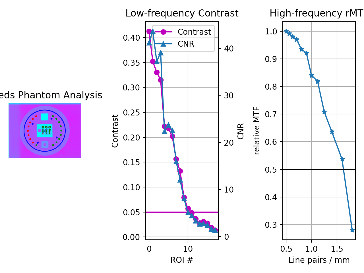
A figure showing the phantom, low contrast plot, and RMTF will be generated:

(Source code, png, hires.png, pdf)

Typical Use¶

Import the class:

from pylinac import (
    LeedsTOR,
)  # or whatever phantom you like from the planar imaging module

The minimum needed to get going is to:

Load image – Load the planar image as you would any other class: by passing the path directly to the constructor:
```
leeds = LeedsTOR("my/leeds.dcm")
```
Alternatively, a URL can be passed:
```
leeds = LeedsTOR.from_url("http://myserver.com/leeds")
```
You may also use the demo image:
```
leeds = LeedsTOR.from_demo_image()
```
Analyze the images – Analyze the image using the analyze() method. The low and high contrast thresholds can be specified:
```
leeds.analyze(low_contrast_threshold=0.01, high_contrast_threshold=0.5)
```
Additionally, you may specify the SSD of the phantom. By default, SAD and 5cm up from SID are searched:
```
leeds.analyze(..., ssd=1400)
```
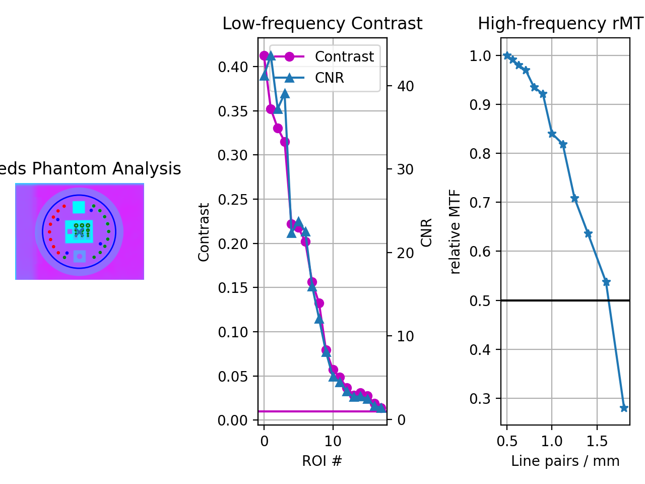
View the results – The results of analysis can be viewed with the plot_analyzed_image() method.
```
leeds.plot_analyzed_image()
```
(Source code, png, hires.png, pdf)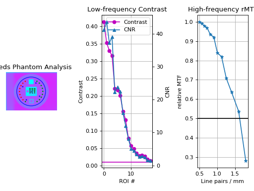

Note that each subimage can be turned on or off.
```
# don't show the low contrast plot
leeds.plot_analyzed_image(low_contrast=False)
```
The figure can also be saved:
```
leeds.save_analyzed_image("myprofile.png")
```
A PDF report can also be generated:
```
leeds.publish_pdf("leeds_october16.pdf")
```

Leeds TOR Phantom¶

The Leeds phantom is used to measure image quality metrics for the kV imager of a linac. It contains both high and low contrast ROIs.

Note

There are two phantom analysis routines. The LeedsTOR class is for newer phantoms that have a red ring on the outside. Older Leeds phantoms may have a blue label containing the serial number and model on the back. Use the LeedsTORBlue class for these phantoms. The difference is small ROI location shifts.

Image Acquisition¶

You can acquire the images any way you like. Just ensure that the phantom is not touching a field edge. It is also recommended by the manufacturer to rotate the phantom to a non-cardinal angle so that pixel aliasing does not occur for the high-contrast line pairs.

Algorithm¶

Leeds phantom analysis is straightforward: find the phantom in the image, then sample ROIs at the appropriate locations.

The algorithm works like such:

Allowances

The images can be acquired at any SID.
The images can be acquired with any size kV imager.
The phantom can be at any distance.
The phantom can be at any angle.
The phantom can be flipped either way.

Restrictions

Warning

Analysis can fail or give unreliable results if any Restriction is violated.

The phantom must not be touching or close to any image edges.
The blades should be fully or mostly open to correctly invert the image. This may not result in a complete failure, but you may have to force-invert the analysis if this case isn’t true (i.e. myleeds.analyze(invert=True)).
The phantom should be centered near the CAX (<1-2cm).

Pre-Analysis

Determine phantom location – The Leeds phantom is found by performing a Canny edge detection algorithm to the image. The thin structures found are sifted by finding appropriately-sized ROIs. This may include the outer phantom edge and the metal ring just inside. The average central position of the circular ROIs is set as the phantom center.
Determine phantom angle – To find the rotational angle of the phantom, a similar process is employed, but square-like features are searched for in the edge detection image. Because there are two square areas, the ROI with the highest attenuation (lead) is chosen. The angle between the phantom center and the lead square center is set as the angle.
Determine rotation direction – The phantom might be placed upside down. To keep analysis consistent, a circular profile is sampled at the radius of the low contrast ROIs starting at the lead square. Peaks are searched for on each semicircle. The side with the most peaks is the side with the higher contrast ROIs. Analysis is always done counter-clockwise. If the ROIs happen to be clockwise, the image is flipped left-right and angle/center inverted.

Analysis

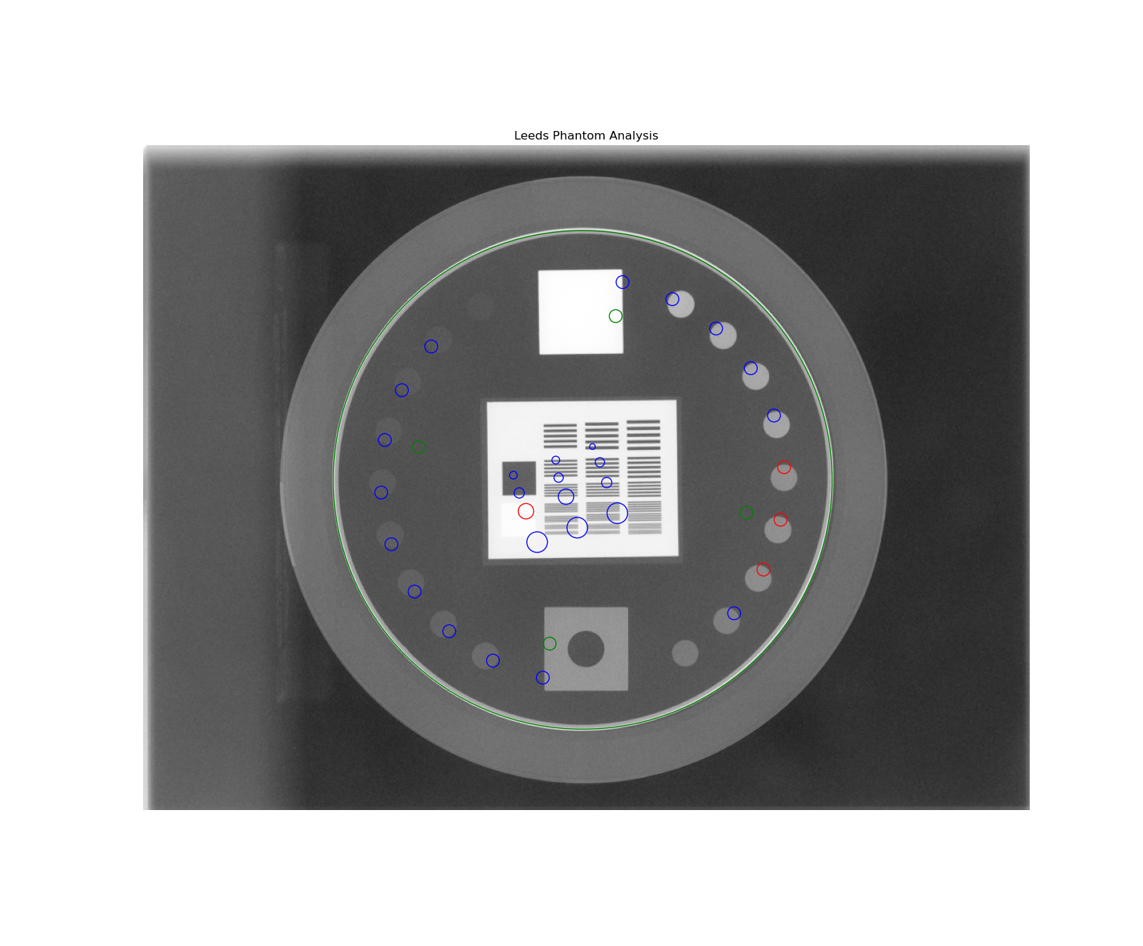
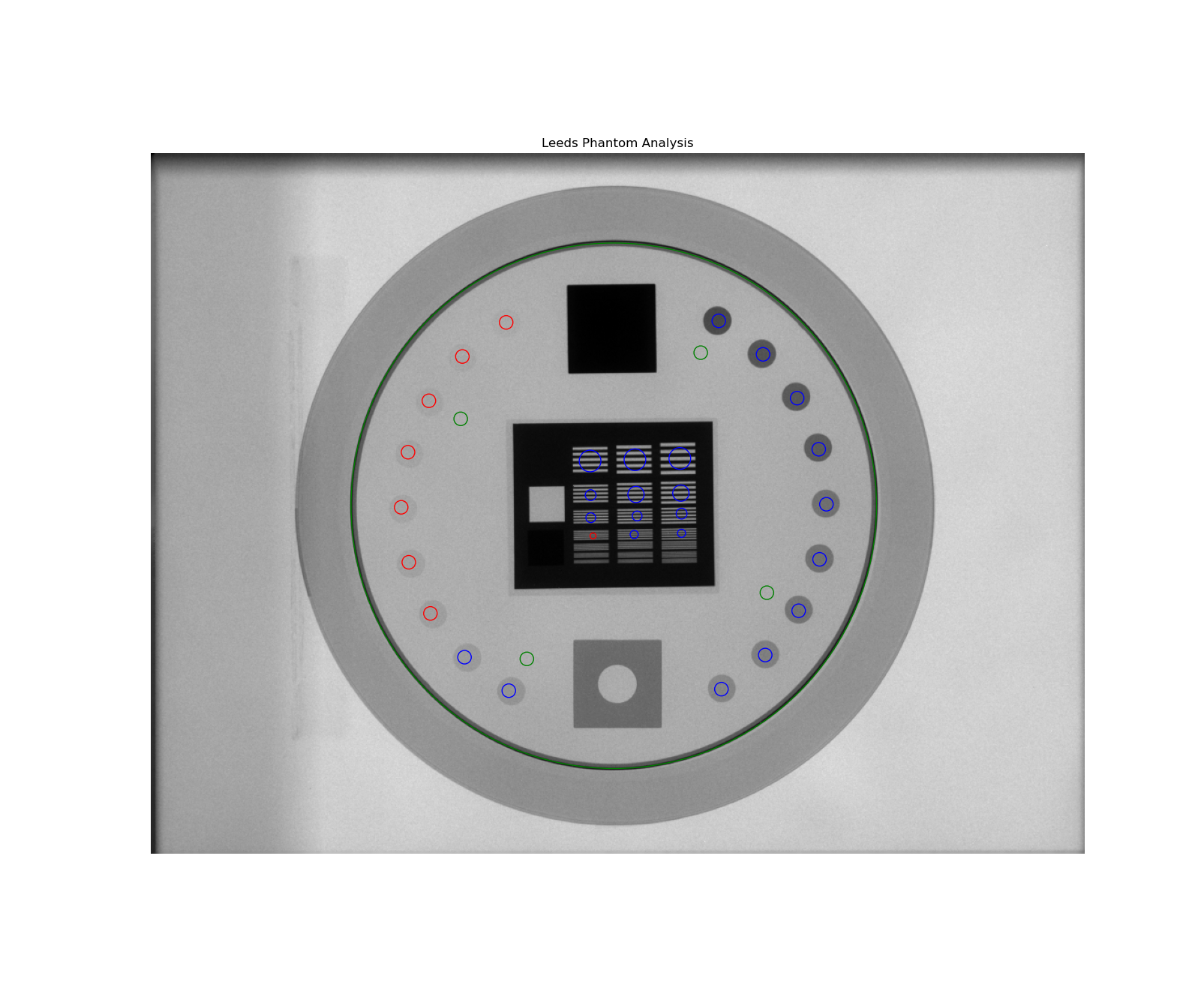
Calculate low contrast – Because the phantom center and angle are known, the angles to the ROIs can also be known. The mean pixel value of each ROI (see below image, “LC0”, …, “LC17”) is compared to the mean pixel value of all 4 reference ROIs (“LCR0”, …, “LCR3”). See also Low contrast. By default, the Michelson algorithm is used. For example, the first contrast value would be calculated as:

\[\frac{LC0_{mean} - LCR_{mean}}{LC0_{mean} + LCR_{mean}}\]
Calculate high contrast – Again, because the phantom position and angle are known, offsets are applied to sample the high contrast line pair regions. For each sample (“HC0”, …, “HC11”), the relative MTF is calculated using Peak-Valley methodology. See Peak-Valley MTF. For example, the first high-contrast value would be calculated as:

\[\frac{HC0_{max} - HC0_{min}}{HC0_{max} + HC0_{min}}\]
Percent Integral Uniformity – See Percent Integral Uniformity.

Post-Analysis

Determine passing low and high contrast ROIs – For each low and high contrast region, the determined value is compared to the threshold. The plot colors correspond to the pass/fail status.

See also Interpreting Results for specific results items.

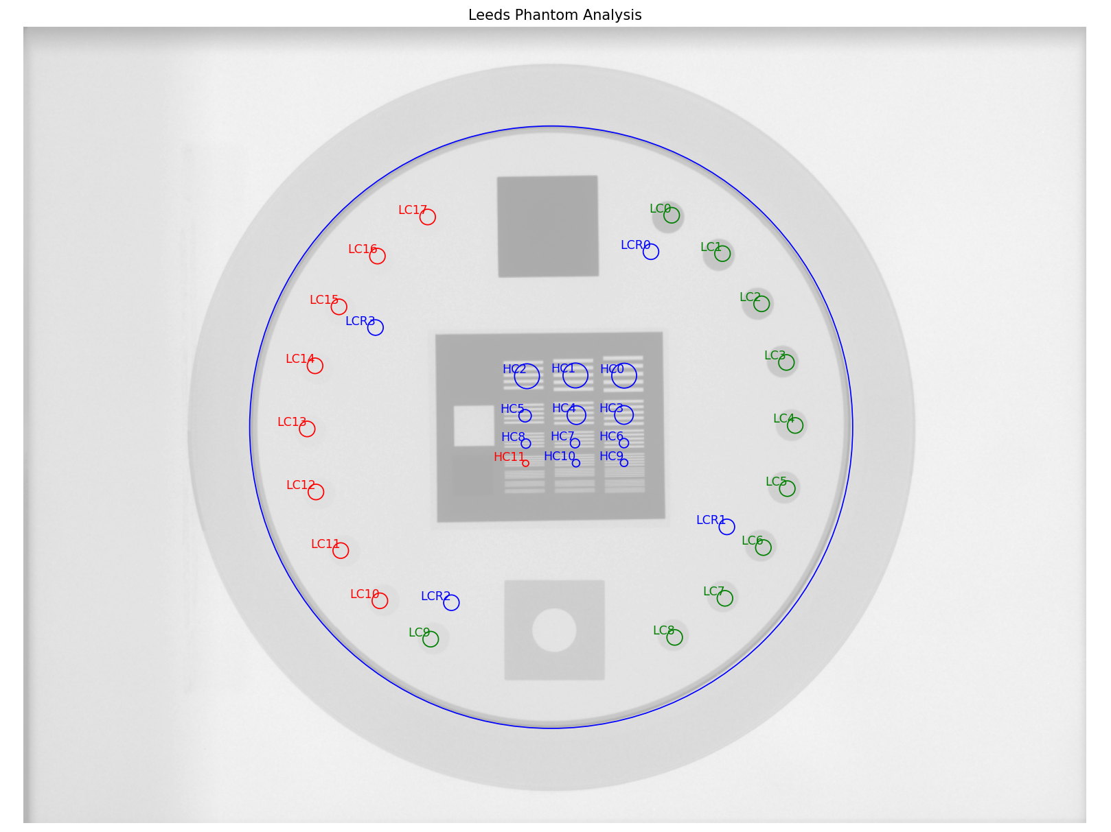
_images/leeds-reference.png — Labeled ROIs of the Leeds phantom analysis. W/L was adjusted for clarify of the labels.¶

Troubleshooting¶

If you’re having trouble getting the Leeds phantom analysis to work, first check out the Troubleshooting section. If the issue is not listed there, then it may be one of the issues below.

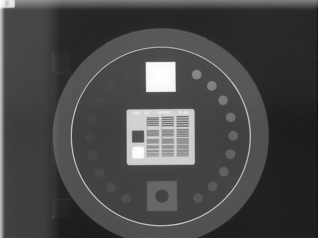
The most common reason for failing is having the phantom near an image edge. The resulting error is usually that the phantom angle cannot be determined. For example, this image would throw an error:

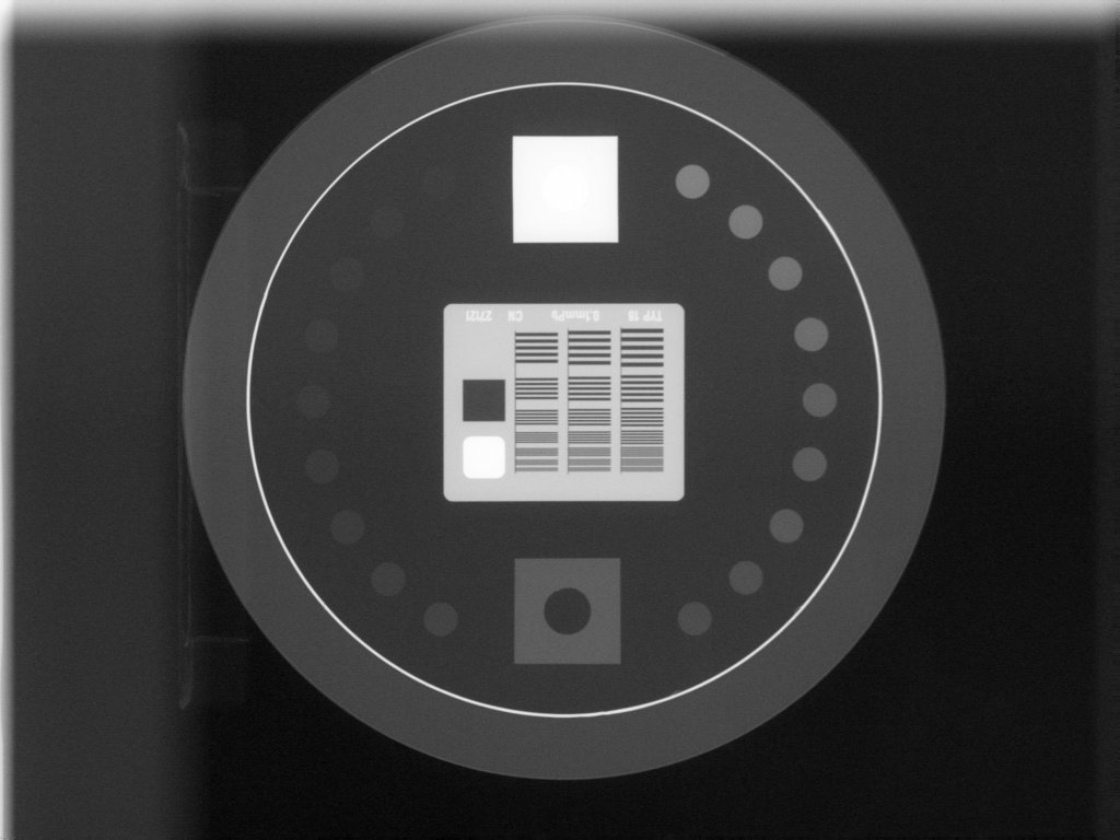
The below image also fails. Technically, the phantom is in the image, but the top blade skews the pixel values such that the phantom edge cannot be properly found at the top. This fails to identify the true phantom edge, causing the angle to also not be found:

Another problem is that the image may have a non-uniform background. This can cause pylinac’s automatic inversion correction to incorrectly invert the image. For example, this image falsely inverts:

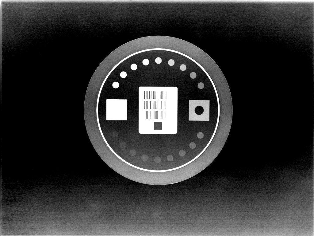
When analyzed, the angle is 180 degrees opposite the lead square, causing the ROIs to be flipped 180 degrees. To correct this problem, pass invert=True to analyze(). This will force pylinac to invert the image the opposite way and correctly identify the lead square.

Another common problem is an offset analysis, as shown below:

This is caused by a wrong inversion.

Note

If the image flash is dark, then the image inversion is very likely wrong.

Again, pass invert=True to the analyze method. This is the same image but with invert=True:

PTW EPID QC Phantom¶

The PTW EPID QC phantom is an MV imaging quality assurance phantom and has high and low contrast regions, just as the Leeds phantom, but with different geometric configurations.

Image Acquisition¶

The EPID QC phantom appears to have a specific setup as recommended by the manufacturer. The phantom should have the high-contrast line pairs at the top of the image and low contrast at the bottom. The rotation is not automatically determined, so you should take care when setting up the phantom to be well-positioned.

Algorithm¶

The algorithm works like such:

Allowances

The images can be acquired at any SID.
The images can be acquired with any EPID.
The images can be acquired with the phantom at any SSD.

Restrictions

Warning

Analysis can fail or give unreliable results if any Restriction is violated.

The phantom must be at 0 degrees.
The phantom must not be touching any image edges.
The phantom should have the high-contrast linen pair regions toward the gantry stand/top.
The phantom should be centered near the CAX (<1-2cm).

Pre-Analysis

Determine phantom location – A Canny edge search is performed on the image. Connected edges that are semi-round and angled are thought to possibly be the phantom. Of the ROIs, the one with the longest axis is said to be the phantom edge. The center of the bounding box of the ROI is set as the phantom center.
Determine phantom radius – The major axis length of the ROI determined above serves as the phantom radius.

Analysis

Calculate low contrast – Because the phantom center and angle are known, the angles to the ROIs can also be known. The mean pixel value of each ROI (see below image, “LC0”, …, “LC8”) is compared to the mean pixel value of the reference ROI (“LCR”). See also Low contrast. By default, the Michelson algorithm is used. For example, the first contrast value would be calculated as:

\[\frac{LC0_{mean} - LCR_{mean}}{LC0_{mean} + LCR_{mean}}\]
Calculate high contrast – Again, because the phantom position and angle are known, offsets are applied to sample the high contrast line pair regions. For each sample (“HC0”, …, “HC6”), the relative MTF is calculated using Peak-Valley methodology. See Peak-Valley MTF. For example, the first high-contrast value would be calculated as:

\[\frac{HC0_{max} - HC0_{min}}{HC0_{max} + HC0_{min}}\]
Percent Integral Uniformity – See Percent Integral Uniformity.

Post-Analysis

Determine passing low and high contrast ROIs – For each low and high contrast region, the determined value is compared to the threshold. The plot colors correspond to the pass/fail status.

See also Interpreting Results for specific results items.

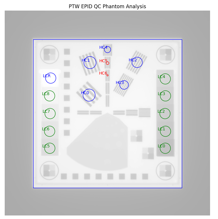
_images/ptw-epid-qc-reference.png — Labeled ROIs of the PTW EPID QC phantom analysis. W/L was adjusted for clarify of the labels.¶

Standard Imaging QC-3 Phantom¶

The Standard Imaging phantom is an MV imaging quality assurance phantom and has high and low contrast regions, just as the Leeds phantom, but with different geometric configurations.

Image Acquisition¶

The Standard Imaging phantom has a specific setup as recommended by the manufacturer. The phantom should be angled 45 degrees, with the “1” pointed toward the gantry stand and centered along the CAX. For best results when using pylinac, open the jaws to fully cover the EPID, or at least give 1-2cm flash around the phantom edges.

Warning

If using the acrylic jig that comes with the phantom, place a spacer of at least a few mm between the jig and the phantom. E.g. a slice of foam on each angled edge. This is because the edge detection of the phantom may fail at certain energies with the phantom abutted to the acrylic jig.

Algorithm¶

The algorithm works like such:

Allowances

The images can be acquired at any SID.
The images can be acquired with any EPID.
The images can be acquired with the phantom at any SSD.

Restrictions

Warning

Analysis can fail or give unreliable results if any Restriction is violated.

The phantom must be at 45 degrees.
The phantom must not be touching any image edges.
The phantom should have the “1” pointing toward the gantry stand.
The phantom should be centered near the CAX (<1-2cm).

Pre-Analysis

Determine phantom location – A Canny edge search is performed on the image. Connected edges that are semi-round and angled are thought to possibly be the phantom. Of the ROIs, the one with the longest axis is said to be the phantom edge. The center of the bounding box of the ROI is set as the phantom center.
Determine phantom radius and angle – The major axis length of the ROI determined above serves as the phantom radius. The orientation of the edge ROI serves as the phantom angle.

Analysis

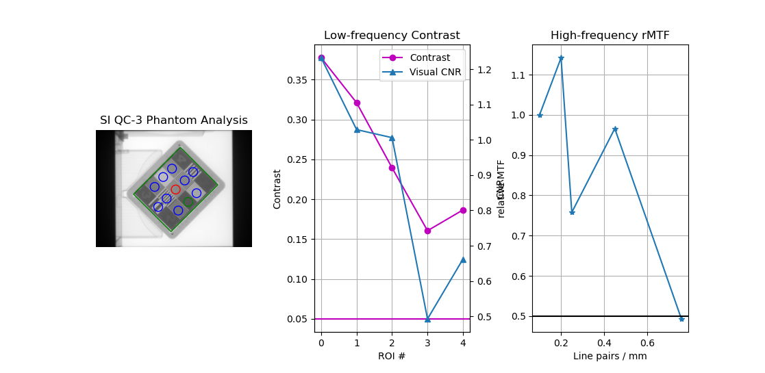
Calculate low contrast – Because the phantom center and angle are known, the angles to the ROIs can also be known. The mean pixel value of each ROI (see below image, “LC0”, …, “LC4”) is compared to the mean pixel value of the reference ROI (“LCR”). See also Low contrast. By default, the Michelson algorithm is used. For example, the first contrast value would be calculated as:

\[\frac{LC0_{mean} - LCR_{mean}}{LC0_{mean} + LCR_{mean}}\]
Calculate high contrast – Again, because the phantom position and angle are known, offsets are applied to sample the high contrast line pair regions. For each sample (“HC0”, …, “HC4”), the relative MTF is calculated using Peak-Valley methodology. See Peak-Valley MTF. For example, the first high-contrast value would be calculated as:

\[\frac{HC0_{max} - HC0_{min}}{HC0_{max} + HC0_{min}}\]
Percent Integral Uniformity – See Percent Integral Uniformity.

Post-Analysis

Determine passing low and high contrast ROIs – For each low and high contrast region, the determined value is compared to the threshold. The plot colors correspond to the pass/fail status.

See also Interpreting Results for specific results items.

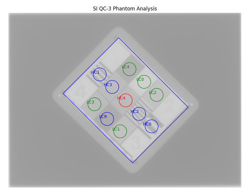
_images/si-qc3-reference.png — Labeled ROIs of the Standard Imaging QC-3 phantom analysis. W/L was adjusted for clarify of the labels.¶

Troubleshooting¶

If you’re having issues with the StandardImaging class, make sure you have correctly positioned the phantom as per the manufacturer’s instructions (also see Image Acquisition). One issue that may arise is incorrect inversion. If the jaws are closed tightly around the phantom, the automatic inversion correction may falsely invert the image, just as for the Leeds phantom. If you have an image that looks inverted or just plain weird, add invert=True to analyze(). If this doesn’t help, reshoot the phantom with the jaws open.

Standard Imaging QC-kV Phantom¶

The Standard Imaging QC-kV phantom is an kV imaging quality assurance phantom and has high and low contrast regions, just as the Leeds phantom, but with different geometric configurations.

Image Acquisition¶

The Standard Imaging phantom has a specific setup as recommended by the manufacturer. The phantom should be angled 45 degrees, with the “1” pointed toward the gantry stand and centered along the CAX. For best results when using pylinac, open the blades to fully cover the kV panel, or at least give 1-2cm flash around the phantom edges.

Warning

Algorithm¶

The algorithm works like such:

Allowances

The images can be acquired at any SID.
The images can be acquired with any kV panel.
The images can be acquired with the phantom at any SSD.

Restrictions

Warning

Analysis can fail or give unreliable results if any Restriction is violated.

The phantom must be at 45 degrees.
The phantom must not be touching any image edges.
The phantom should have the “1” pointing toward the gantry stand.
The phantom should be centered near the CAX (<1-2cm).

Pre-Analysis

Determine phantom location – A Canny edge search is performed on the image. Connected edges that are semi-round and angled are thought to possibly be the phantom. Of the ROIs, the one with the longest axis is said to be the phantom edge. The center of the bounding box of the ROI is set as the phantom center.
Determine phantom radius and angle – The major axis length of the ROI determined above serves as the phantom radius. The orientation of the edge ROI serves as the phantom angle.

Analysis

Calculate low contrast – Because the phantom center and angle are known, the angles to the ROIs can also be known. The mean pixel value of each ROI (see below image, “LC0”, …, “LC4”) is compared to the mean pixel value of the reference ROI (“LCR”). See also Low contrast. By default, the Michelson algorithm is used. For example, the first contrast value would be calculated as:

\[\frac{LC0_{mean} - LCR_{mean}}{LC0_{mean} + LCR_{mean}}\]
Calculate high contrast – Again, because the phantom position and angle are known, offsets are applied to sample the high contrast line pair regions. For each sample (“HC0”, …, “HC4”), the relative MTF is calculated using Peak-Valley methodology. See Peak-Valley MTF. For example, the first high-contrast value would be calculated as:

\[\frac{HC0_{max} - HC0_{min}}{HC0_{max} + HC0_{min}}\]

Post-Analysis

Determine passing low and high contrast ROIs – For each low and high contrast region, the determined value is compared to the threshold. The plot colors correspond to the pass/fail status.

See also Interpreting Results for specific results items.

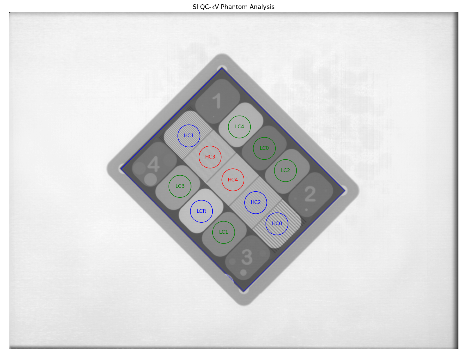
_images/qckv-reference.png — Labeled ROIs of the QC-kV phantom analysis.¶

Troubleshooting¶

Las Vegas Phantom¶

The Las Vegas phantom is for MV image quality testing and includes low contrast regions of varying contrast and size. There is also a ElektaLasVegas class that is very similar. This section covers both styles.

Image Acquisition¶

The Las Vegas phantom has a recommended position as stated on the phantom. Pylinac will however account for shifts and inversions. Best practices for the Las Vegas phantom:

Keep the phantom from a couch edge or any rails.
The field edge should be >=5mm from the phantom edge, preferably 10+mm.
The orientation should have the largest “holes” towards the right side although this can be accounted for as an analyze parameter.
The angle should be as close to 0 as possible, given above, although this can be accounted for as an analyze parameter.

Algorithm¶

The algorithm works like such:

Allowances

The images can be acquired at any SID.
The images can be acquired with any EPID.

Restrictions

Warning

Analysis can fail or give unreliable results if any Restriction is violated.

The phantom must not be touching any image edges.
The phantom should be at a cardinal angle (0, 90, 180, or 270 degrees) relative to the EPID.
The phantom should be centered near the CAX (<1-2cm).

Pre-Analysis

Determine phantom location – A Canny edge search is performed on the image. Connected edges that are semi-round and angled are thought to possibly be the phantom. Of the ROIs, the one with the longest axis is said to be the phantom edge. The center of the bounding box of the ROI is set as the phantom center.
Determine phantom radius and angle – The major axis length of the ROI determined above serves as the phantom radius. The orientation of the edge ROI serves as the phantom angle.

Analysis

Calculate low contrast – Because the phantom center and angle are known, the angles to the ROIs can also be known. The mean pixel value of each ROI (see below image, “LC0”, …, “LC18”) is compared to the mean pixel value of all 4 reference ROIs (“LCR0”, …, “LCR3”). See also Low contrast. By default, the Michelson algorithm is used. For example, the first contrast value would be calculated as:

\[\frac{LC0_{mean} - LCR_{mean}}{LC0_{mean} + LCR_{mean}}\]

Post-Analysis

Determine passing low and high contrast ROIs – For each low and high contrast region, the determined value is compared to the threshold. The plot colors correspond to the pass/fail status.

See also Interpreting Results for specific results items.

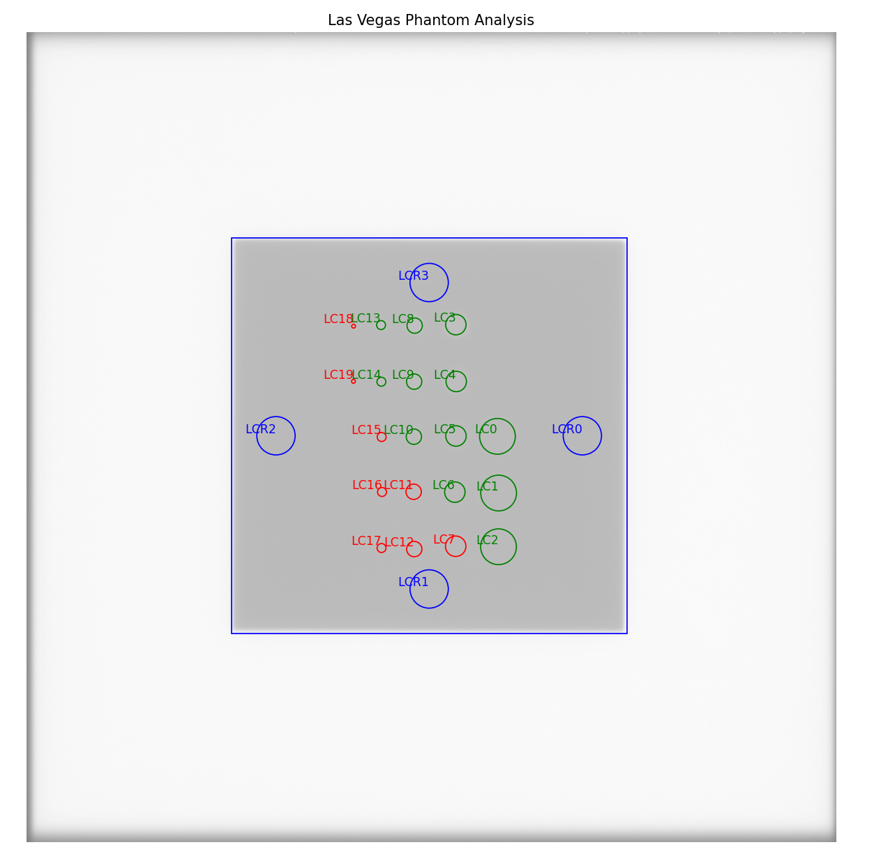
_images/las-vegas-reference.png — Labeled ROIs of the Las Vegas phantom analysis. W/L was adjusted for clarify of the labels.¶

Doselab MC2 MV & kV¶

The Doselab MC2 phantom is for both kV & MV image quality testing and includes low and high contrast regions of varying contrast. There are two high contrast sections, one intended for kV and one for MV.

Image Acquisition¶

The Doselab phantom has a recommended position as stated on the phantom. Pylinac will however account for shifts and inversions. Best practices for the Doselab phantom:

Keep the phantom away from a couch edge or any rails.
Center the phantom along the CAX.

Algorithm¶

The algorithm works like such:

Allowances

The images can be acquired at any SID.
The images can be acquired with any EPID.

Restrictions

Warning

Analysis can fail or give unreliable results if any Restriction is violated.

The phantom must not be touching any image edges.
The phantom should be at 45 degrees relative to the EPID.
The phantom should be centered near the CAX (<1-2cm).

Pre-Analysis

Determine phantom location – A canny edge search is performed on the image. Connected edges that are semi-round and angled are thought to possibly be the phantom. Of the ROIs, the one with the longest axis is said to be the phantom edge. The center of the bounding box of the ROI is set as the phantom center.
Determine phantom radius and angle – The major axis length of the ROI determined above serves as the phantom radius. The orientation of the edge ROI serves as the phantom angle.

Analysis

Calculate low contrast – Because the phantom center and angle are known, the angles to the ROIs can also be known. The mean pixel value of each ROI (see below image, “LC0”, …, “LC6”) is compared to the mean pixel value of the reference ROI (“LCR”). See also Low contrast. By default, the Michelson algorithm is used. For example, the first contrast value would be calculated as:

\[\frac{LC0_{mean} - LCR_{mean}}{LC0_{mean} + LCR_{mean}}\]
Calculate high contrast – Again, because the phantom position and angle are known, offsets are applied to sample the high contrast line pair regions. For each sample (“HC0”, …, “HC3”), the relative MTF is calculated using Peak-Valley methodology. See Peak-Valley MTF. For example, the first high-contrast value would be calculated as:

\[\frac{HC0_{max} - HC0_{min}}{HC0_{max} + HC0_{min}}\]

Post-Analysis

Determine passing low and high contrast ROIs – For each low and high contrast region, the determined value is compared to the threshold. The plot colors correspond to the pass/fail status.

See also Interpreting Results for specific results items.

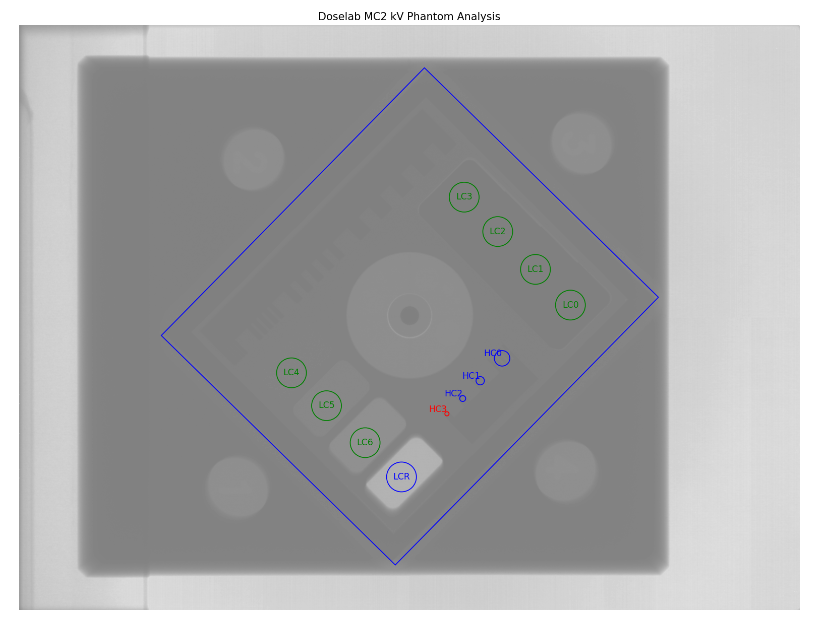
_images/doselab-kv-reference.png — Labeled ROIs of the Doselab MC2 kV phantom analysis. W/L was adjusted for clarify of the labels.¶

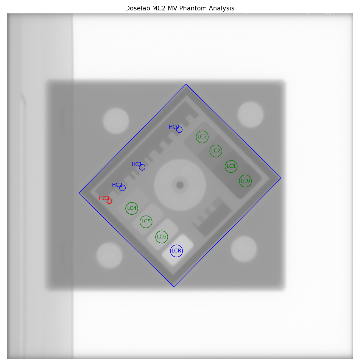
_images/doselab-mv-reference.png — Labeled ROIs of the Doselab MC2 MV phantom analysis. W/L was adjusted for clarify of the labels.¶

SNC MV & kV¶

The SNC MV and kV phantoms are for kV & MV image quality testing and includes low and high contrast regions of varying contrast.

Image Acquisition¶

The SNC phantoms typically use the angled setup jig. Best practices for the Doselab phantom:

Keep the phantom away from a couch edge or any rails.
Center the phantom along the CAX.
Use the angled setup jig.
For the MV phantom, have the longer side point inferiorly (i.e. away from the stand).
For the kV phantom, have the longer side point superiorly (i.e. toward the stand).

Algorithm¶

The algorithm works like such:

Allowances

The images can be acquired at any SID.
The images can be acquired with any EPID.

Restrictions

Warning

Analysis can fail or give unreliable results if any Restriction is violated.

The phantom must not be touching any image edges.
The phantom should be at 45 degrees relative to the EPID.
The phantom should be centered near the CAX (<1-2cm).

Pre-Analysis

Determine phantom location – A canny edge search is performed on the image. Connected edges that are semi-round and angled are thought to possibly be the phantom. Of the ROIs, the one with the longest axis is said to be the phantom edge. The center of the bounding box of the ROI is set as the phantom center.
Determine phantom radius – The major axis length of the ROI determined above serves as the phantom radius.

Analysis

Calculate low contrast – Because the phantom center and angle are known, the angles to the ROIs can also be known. The mean pixel value of each ROI (see below image, “LC0”, …, “LC3”) is compared to the mean pixel values of both of the reference ROIs (“LCR0”, “LCR1”). See also Low contrast. By default, the Michelson algorithm is used. For example, the first contrast value would be calculated as:

\[\frac{LC0_{mean} - LCR_{mean}}{LC0_{mean} + LCR_{mean}}\]
Calculate high contrast – Again, because the phantom position and angle are known, offsets are applied to sample the high contrast line pair regions. For each sample (“HC0”, …, “HC3”), the relative MTF is calculated using Peak-Valley methodology. See Peak-Valley MTF. For example, the first high-contrast value would be calculated as:

\[\frac{HC0_{max} - HC0_{min}}{HC0_{max} + HC0_{min}}\]

Post-Analysis

Determine passing low and high contrast ROIs – For each low and high contrast region, the determined value is compared to the threshold. The plot colors correspond to the pass/fail status.

See also Interpreting Results for specific results items.

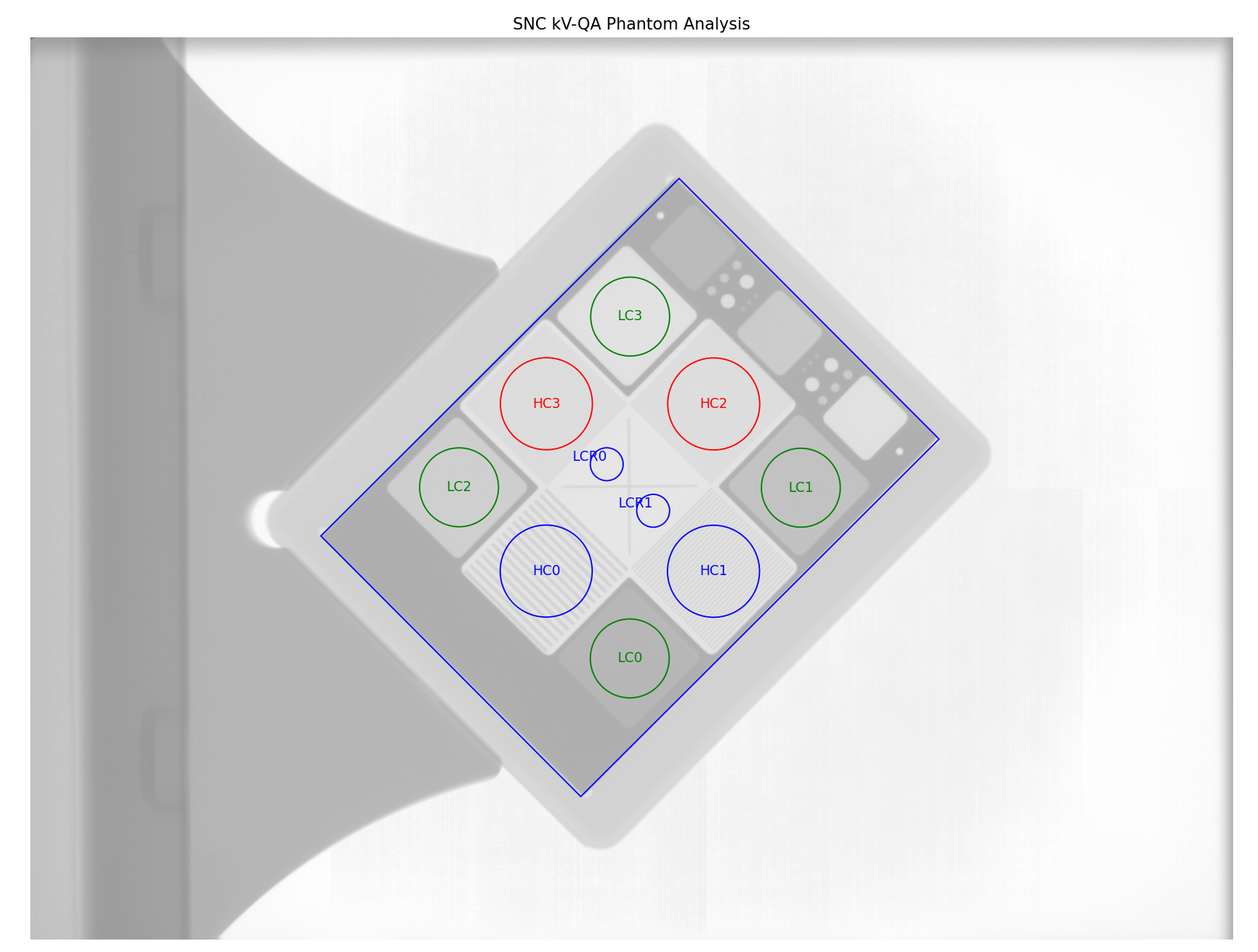
_images/snc-kv-reference.png — Labeled ROIs of the SNC kV phantom analysis. W/L was adjusted for clarify of the labels.¶

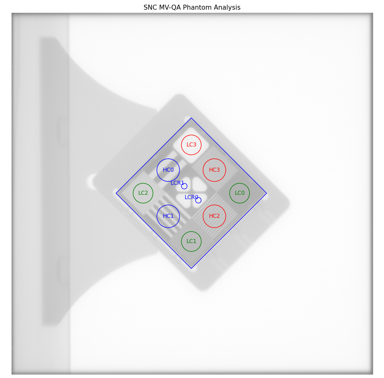
_images/snc-mv-reference.png — Labeled ROIs of the SNC MV phantom analysis. W/L was adjusted for clarify of the labels.¶

IBA Primus A¶

The IBA Primus A phantom is used for kV image analysis and includes low and high contrast regions of varying contrast.

Image Acquisition¶

Lay the phantom on the couch with the wedge step circle facing the top/gun and high-res square facing the bottom/target.

Algorithm¶

The algorithm works like such:

Allowances

The images can be acquired at any SID.
The images can be acquired with any EPID.

Restrictions

Warning

Analysis can fail or give unreliable results if any Restriction is violated.

The phantom must not be touching any image edges.
The phantom should be at 0, 90, or 270 +/-5 degrees relative to the EPID where 0 is facing the gun.
The dynamic wedge steps should be facing the gun side; the high-resolution square should be facing the target side.
The phantom should be centered near the CAX (<2cm).

Pre-Analysis

Determine phantom location – A Canny edge search is performed on the image. The ROI that approximates the size of the central crosshair of the phantom and is nearly at the center of the image is used as the phantom center location
Determine phantom radius – The size of the above crosshair ROI is used as the basis for the phantom radius.
Fine-tune phantom angle – The phantom angle is assumed to be around 0 (wedge steps facing gun), but fine-tuning is performed so that sensitive ROIs like MTF can be had with high accuracy. This is performed by taking a circular profile about the phantom at the radius of the wedge steps. The two areas of highest gradient will be at the first and last wedge steps. The center between these two points is the angle at which the phantom is “pointing” and will be used as the updated angle.

Warning

If the gradients cannot be found or if the determined angle is >5 degrees (caused by bad inversion, e.g.) a warning will be printed to the console and a default of 0 will be used.

Analysis

Calculate low contrast – Because the phantom center and angle are known, the angles to the ROIs can also be known. The mean pixel value of each ROI (see below image, “LC0”, …, “LC14”) is compared to the mean pixel values of the reference ROI (“LCR”). See also Low contrast. By default, the Michelson algorithm is used. For example, the first contrast value would be calculated as:

\[\frac{LC0_{mean} - LCR_{mean}}{LC0_{mean} + LCR_{mean}}\]
Calculate high contrast – Again, because the phantom position and angle are known, offsets are applied to sample the high contrast line pair regions. For each sample (“HC0”, …, “HC12”), the relative MTF is calculated using Peak-Valley methodology. See Peak-Valley MTF. For example, the first high-contrast value would be calculated as:

\[\frac{HC0_{max} - HC0_{min}}{HC0_{max} + HC0_{min}}\]

Post-Analysis

Determine passing low and high contrast ROIs – For each low and high contrast region, the determined value is compared to the threshold. The plot colors correspond to the pass/fail status.

See also Interpreting Results for specific results items.

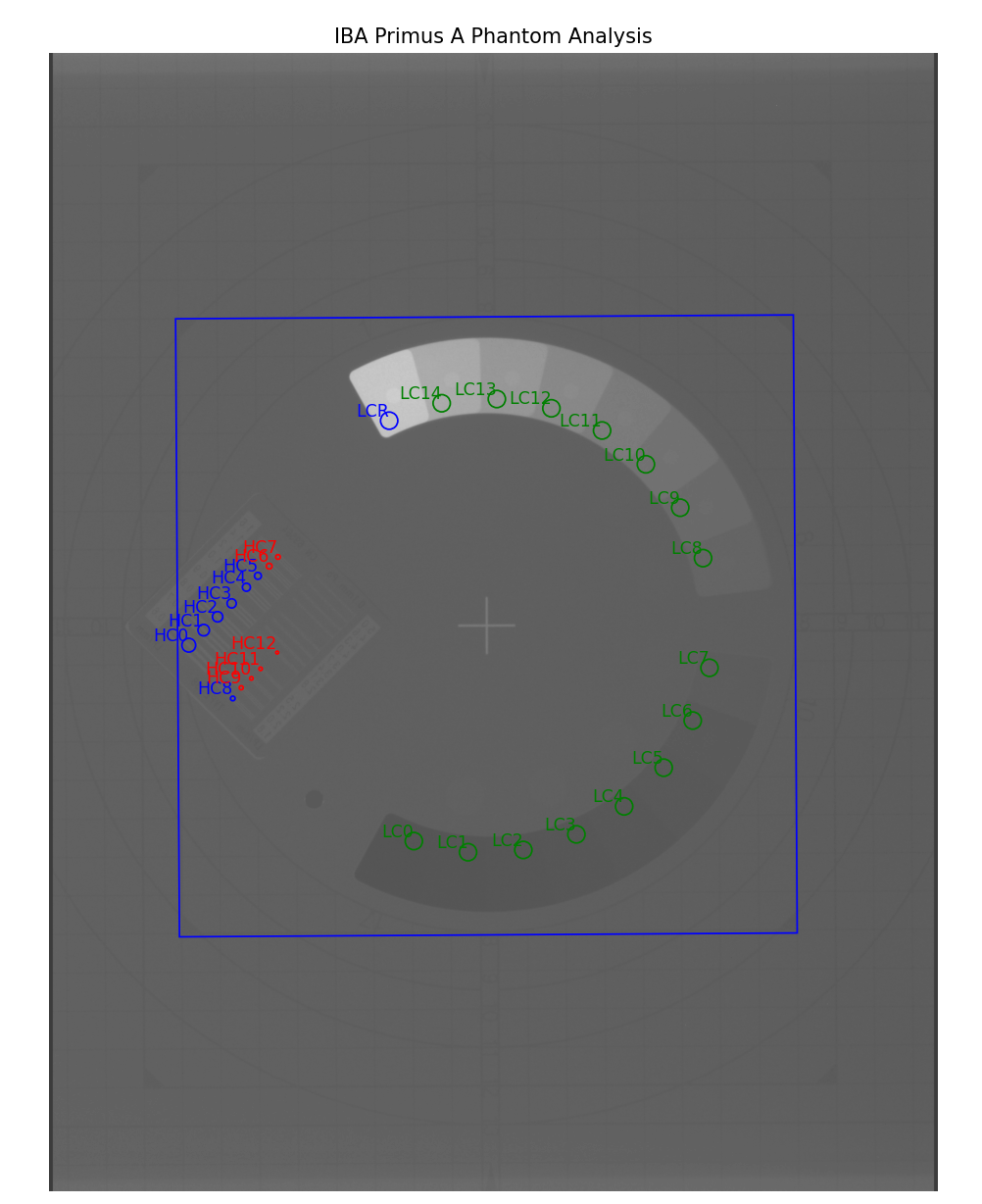
_images/iba-primus-a-reference.png — Labeled ROIs of the IBA Primus A phantom analysis.¶

ACR Digital Mammography¶

Warning

This phantom analysis is still in beta. The parameters may change in future releases.

The ACR Digital Mammography phantom is for testing the performance of Full-Field Digital Mammography (FFDM) systems.

Image Acquisition¶

The ACR Digital Mammography phantom has a recommended position as stated on ACR Phantom Testing: Mammography (Revised 11-22-2024)

Best practices for the ACR Digital Mammography phantom:

Place the chest-wall side of phantom completely flush with chest-wall side of image receptor.
Small deviations from being flush can be accounted for using angle_adjustment, x_adjustment, and y_adjustment in the analyze parameter.

Algorithm¶

Pre-Analysis

Determine phantom location – A Canny edge search is performed on the image. Connected edges that are semi-round and angled are thought to possibly be the phantom. Of the ROIs, the one closest to the expected area is said to be the phantom edge. The center of the bounding box of the ROI is set as the phantom center.

Analysis

The ACR Digital Mammography phantom is composed of 3 test objects: Masses, Speck groups, and Fibers.

Calculate masses – Because the phantom center and angle are known, the angles to the ROIs can also be known. The mean pixel value of each ROI is compared to the mean pixel value of the reference ROIs. See also Low contrast. By default, the Michelson algorithm is used. For example, the first contrast value would be calculated as:

\[\frac{LC0_{mean} - LCR_{mean}}{LC0_{mean} + LCR_{mean}}\]
Calculate speck groups – Because the phantom center and angle are known, the positions to the center of the speck groups can also be known. Furthermore, since the individual specks within a group follow the vertices of a pentagon, their positions can also be know. The visibility of the individual specks is evaluated with a variation of the Visibility algorithm

\[Visibility(I, R) = Contrast(I, R) * \frac{\sqrt{\pi * radius^2}}{R_{std}}\]

where I is the max intensity in the ROI, R is the mean signal of the ROI, \(R_{std}\) is the standard deviation of the ROI, and radius is the radius of the speck per manual description. By default, the Weber algorithm is used for Contrast.
Calculate fibers – Because the phantom center and angle are known, the positions to the fibers can also be known. A fiber is detected using a sequence of image processing filters:
1. Vesselness filter – uses the Frangi filter to detect vessel-like structures.
2. Thresholding – convert to binary.
3. Closing – connects parts of a fiber if there are breaks.
4. Label – detect connected blobs.
5. Regionprops – detect the blob most likely to be the fiber.
6. Length – calculate the length of the fiber as the length of the major axis of the ellipse in regionprops.

Standard Imaging FC-2¶

The FC-2 phantom is for testing light/radiation coincidence.

Image Acquisition¶

The FC-2 phantom should be placed on the couch at 100cm SSD.

Keep the phantom away from a couch edge or any rails.

Algorithm¶

The algorithm works like such:

Allowances

The images can be acquired at any SID.
The images can be acquired with any EPID.

Restrictions

Warning

Analysis can fail or give unreliable results if any Restriction is violated.

The phantom should be at a cardinal angle (0, 90, 180, or 270 degrees) relative to the EPID.
The phantom should be centered near the CAX (<1cm).
The phantom should be +/- 1cm from 100cm SSD.

Pre-Analysis

Determine BB set to use – There are two sets of BBs, one for 10x10cm and another for 15x15cm. To get the maximum accuracy, the larger set is used if a 15x15cm field is irradiated. The field size is determined and if it’s >14cm then the algorithm will look for the larger set. Otherwise, it will look for the smaller 4.

Analysis

Get BB centroid – Once the BB set is chosen, image windows look for the BBs in a 1x1cm square. Once it finds them, the centroid of all 4 BBs is calculated.
Determine field center – The field size is measured along the center of the image in the inplane and crossplane direction. A 5mm strip is averaged and used to reduce noise.

Post-Analysis

Comparing centroids – The irradiated field centroid is compared to the EPID/image center as well as the the BB centroid. The field size is also reported.

Doselab RLf¶

Added in version 3.15.

The Doselab RLf is for testing light/radiation coincidence. See also DoselabRLf.

Image Acquisition¶

The RLf phantom should be placed on the couch at 100cm SSD.

Keep the phantom away from a couch edge or any rails.

Algorithm¶

The algorithm works like such:

Allowances

The images can be acquired at any SID.
The images can be acquired with any EPID.

Restrictions

Warning

Analysis can fail or give unreliable results if any Restriction is violated.

The phantom should be at a cardinal angle (0, 90, 180, or 270 degrees) relative to the EPID.
The phantom should be centered near the CAX (<2mm).

Analysis

Get BB centroid – An image window looks for each BB on the inner side of each edge. After finding the BBs, the centroid is calculated.

Note

The inner 10x10 BBs are always used regardless of the field size. This is because the BB detection is more robust when the BBs are away from a field edge. This also means that 10x10 analysis is slightly less robust that 15x15 analysis all else being equal.
Determine field center – The field size is measured along the center of the image in the inplane and crossplane direction. A 5mm strip is averaged and used to reduce noise.

Post-Analysis

Comparing centroids – The irradiated field centroid is compared to the EPID/image center as well as the the BB centroid. The field size is also reported.

IsoAlign¶

Added in version 3.15.

The IsoAlign phantom is for testing light/radiation coincidence. See also IsoAlign.

Image Acquisition¶

The phantom should be placed on the couch at 100cm SSD.

Keep the phantom away from a couch edge or any rails.

Algorithm¶

The algorithm works like such:

Allowances

The images can be acquired at any SID.
The images can be acquired with any EPID.

Restrictions

Warning

Analysis can fail or give unreliable results if any Restriction is violated.

The phantom should be at a cardinal angle (0, 90, 180, or 270 degrees) relative to the EPID.
The phantom should be centered near the CAX (<2mm).

Analysis

Get BB centroid – An image window looks for the central BB as well as 1 BB in each cardinal direction. After finding the BBs, the centroid is calculated.
Determine field center – The field size is measured along the center of the image in the inplane and crossplane direction. A 10mm strip is averaged and used to reduce noise.

Post-Analysis

Comparing centroids – The irradiated field centroid is compared to the EPID/image center as well as the the BB centroid. The field size is also reported.

IMT L-Rad¶

Added in version 3.2.

The IMT L-Rad phantom is for testing light/radiation coincidence. Unlike the FC-2 phantom, the L-Rad’s BBs are all the way at the edge of the phantom. This means for any size below 20x20cm those BBs can’t be seen. Even at 20x20, the field edge partially obscures the BBs. For this reason, we only use the central BB for detection.

Image Acquisition¶

The L-Rad phantom should be placed on the couch at 100cm SSD.

Keep the phantom away from a couch edge or any rails.

Algorithm¶

The algorithm works like such:

Allowances

The images can be acquired at any SID.
The images can be acquired with any EPID.

Restrictions

Warning

Analysis can fail or give unreliable results if any Restriction is violated.

The phantom should be at a cardinal angle (0, 90, 180, or 270 degrees) relative to the EPID.
The phantom should be centered near the CAX (<3mm).

Analysis

Get BB centroid – An image window looks for the central BB in a 1.2x1.2cm square. Once it finds it, the centroid is calculated.
Determine field center – The field size is measured along the center of the image in the inplane and crossplane direction. A 5mm strip is averaged and used to reduce noise.

Post-Analysis

Comparing centroids – The irradiated field centroid is compared to the EPID/image center as well as the the BB centroid. The field size is also reported.

SNC FSQA¶

Added in version 3.3.

The SNC FSQA phantom is for light/radiation coincidence. It contains markers which guide the physicist on how to position the light field for either a 10x10 or 15x15cm field. There is also an offset BB 4cm at the top right of the image. Because of both the philosophy of pylinac on light/rad and also because pylinac is a library and not a GUI, there is no interaction to find the edge markers. Instead, we use the one offset BB and then offset that point back 4cm in each direction to get a “virtual center”. This center is compared to the field center and EPID center. The expectation is that the physicist set up their field to the markers using the light field at the time of acquisition.

Image Acquisition¶

The FSQA phantom should be placed on the couch at 100cm SSD.

Keep the phantom away from a couch edge or any rails.
Keep the phantom as close to 0 degrees rotation as possible.

Algorithm¶

The algorithm works like such:

Allowances

The images can be acquired at any SID.
The images can be acquired with any EPID.

Restrictions

Warning

Analysis can fail or give unreliable results if any Restriction is violated.

The phantom should be at 0 degrees relative to the EPID.
The phantom should be roughly centered along the CAX (<3mm).

Analysis

Get BB centroid – An image window looks for the top-right offset BB in a 1.2x1.2cm square. Once it finds it, a “virtual center” centroid is calculated by shifting the detected BB location by 4cm in each direction.
Determine field center – The field size is measured along the center of the image in the inplane and crossplane direction. A 5mm strip is averaged and used to reduce noise.

Post-Analysis

Comparing centroids – The irradiated field centroid is compared to the EPID/image center as well as the the BB centroid. The field size is also reported.

Analysis Parameters¶

pylinac

See the analyze method of the class. E.g. pylinac.planar_imaging.LasVegas.analyze().

RadMachine

Source-to-Phantom distance: The distance in mm from the phantom to the source.
Normalized high contrast threshold: The rMTF minimum value for a region to be considered passing.
Angle override: The angle in degrees to override the automatic angle determination.
Contrast definition: The method to use to calculate contrast. See Contrast.
Contrast threshold: The minimum contrast value for a region to be considered passing.

Analysis Parameters (Light/Rad)¶

These are the analysis parameters for Light/Rad phantoms.

pylinac

See pylinac.planar_imaging.IMTLRad.analyze() and similar classes for details.

RadMachine

FWXM height: The percent height of the maximum to use as the field width.
BB edge distance threshold: The threshold in mm to determine if the BB is near the edge of the image. If the BB-to-field-edge is less than this threshold, a different, more robust algorithm is used to determine the BB position but results in higher uncertainty when in a flat region (i.e. away from the field edge).

Analysis Parameters (ACR Mammography)¶

These are the analysis parameters for ACR Digital Mammography phantom:

pylinac

See pylinac.planar_imaging.ACRDigitalMammography.analyze() for details.

RadMachine

Source-to-Phantom distance: The distance in mm from the phantom to the source.
Mass Contrast definition: The method to use to calculate contrast for mass ROIs. See Contrast.
Mass Visibility threshold: The minimum contrast value for a mass ROI to be considered passing.
Speck Group Contrast definition: The method to use for calculating the contrast of speck groups.
Speck Group Visibility threshold: The threshold for whether a speck is “seen”.
Speck group half threshold: The speck group score is 0.5 if the number of visible specks is between this value and the full threshold.
Speck group full threshold: The speck group score is 1.0 if the number of visible specks is larger or equal than this value.
Max Fiber gap: The max allowed gap in mm between partial fibers.
Fiber length half threshold: The fiber score is 0.5 if its length is between this value and the full threshold (in mm).
Fiber length full threshold: The fiber score is 1.0 if its length is larger or equal than this value (in mm).
Fiber orientation tolerance: The tolerance in degrees to validate the fiber orientation.
X adjustment: A fine-tuning adjustment to the detected x-coordinate of the phantom center in mm. Positive values move the phantom to the right.
Y adjustment: A fine-tuning adjustment to the detected y-coordinate of the phantom center in mm. Positive values move the phantom down.
Angle adjustment: A fine-tuning adjustment to the detected angle of the phantom in degrees. Positive values rotate the phantom clockwise.
ROI size factor: A fine-tuning adjustment to the ROI sizes. This scales the ROIs by this amount. Positive values increase the ROI sizes.
Scaling factor: A fine-tuning adjustment to the detected magnification of the phantom. This zooms the ROIs and phantom outline by this amount.

Interpreting Results¶

Phantoms¶

The results from phantoms that are meant to measure image quality, contrast, etc, are:

median_contrast: The median contrast of the low contrast ROIs. See Low contrast and Contrast-to-noise ratio for more.
median_cnr: The median contrast-to-noise ratio of the low contrast ROIs.
num_contrast_rois_seen: The number of low contrast ROIs that had a visibility score above the passed threshold. See Visibility for more.
phantom_center_x_y: The center of the phantom in the image in pixels.
phantom_area: The area of the phantom in pixels^2.
mtf_lp_mm: The 80%, 50%, and 30% MTF values in lp/mm. For more values see: Calculate a specific MTF.
percent_integral_uniformity: The percent integral uniformity of the image. See Percent Integral Uniformity.
low_contrast_rois: A dictionary of the individual low contrast ROIs. The dictionary keys are the ROI number, starting at 0. Each ROI has the following information:
- contrast method: The method used to calculate the contrast. See Low contrast.
- contrast: The contrast value of the ROI.
- visibility: The visibility score of the ROI.
- visibility threshold: The threshold used to determine visibility.
- cnr: The contrast-to-noise ratio of the ROI.
- passed visibility: Whether the ROI passed the visibility threshold.
- signal to noise: The signal-to-noise ratio of the ROI.

Light/Rad¶

Light/radiation coincidence phantoms are used to ensure that the light field and radiation field are aligned. The results from these analyses are:

field_size_x_mm: The size of the field in the x-direction/crossplane in mm.
field_size_y_mm: The size of the field in the y-direction/inplane in mm.
field_epid_offset_x_mm: The offset of the field center from the EPID/image center in the x-direction/crossplane in mm.
field_epid_offset_y_mm: The offset of the field center from the EPID/image center in the y-direction/inplane in mm.
field_bb_offset_x_mm: The offset of the field center from the BB center in the x-direction/crossplane in mm.
field_bb_offset_y_mm: The offset of the field center from the BB center in the y-direction/inplane in mm.

Note

Some phantoms have multiple BBs. When we speak of the BB center when multiple BBs are present, we are referring to the centroid of all BBs.

Percent Integral Uniformity¶

The uniformity of the phantom can be found by using the percent_integral_uniformity() method. This uses the same equation as ACR for CT uniformity. See the “Uniformity” section under ACR Analysis for more information.

The PIU is calculated over all the low-contrast ROIs and the lowest (worst) PIU is returned.

For robustness, the 1st and 99th percentiles are used rather than the min/max. The true min/max can be influenced by salt and paper noise. To use the true min and max, set the percentiles to 0 and 100 respectively:

Note

Calls to percent_integral_uniformity will not be reflected in the results_data structure; it will always use (1, 99).

leeds = LeedsTOR(...)
leeds.analyze(...)
print(leeds.percent_integral_uniformity(percentiles=(0, 100)))  # uses the true min/max

Warning

This equation was chosen because it is common and understood, but it does come with pitfalls. It is not designed to handle negative values or 0. The calculated result may be misleading if these conditions exist.

Customizing Light/Rad behavior¶

The BB window as well as the expected BB positions, and field strip size can be overridden like so:

from pylinac import StandardImagingFC2  # works for any light/rad phantom


class MySIFC2(StandardImagingFC2):
    bb_sampling_box_size_mm = (
        20  # look at a 20x20mm window for the BB at the expected position
    )
    # change the 10x10 BB expected positions. This is in mm relative to the CAX.
    bb_positions_10x10 = {
        "TL": [-30, -30],
        "BL": [-30, 30],
        "TR": [30, -30],
        "BR": [30, 30],
    }
    bb_positions_15x15 = ...  # same as above
    field_strip_width_mm = 10  # 10mm strip in x and y to determine field size


# use as normal
fc2 = MySIFC2(...)

Creating a custom planar phantom¶

In the event you would like to analyze a phantom that pylinac does not analyze out of the box, the pylinac planar imaging module structure allows for generating new phantom analysis types quickly and easily. The benefit of this design is that with a few simple definitions you inherit a strong base of methods (e.g. plotting and PDF reports come for free).

Creating a new class involves a few different steps but can be done in a few minutes. The following is a guide for custom phantoms:

Subclass the ImagePhantomBase class:

from pylinac.planar_imaging import ImagePhantomBase


class CustomPhantom(ImagePhantomBase):
    pass

Define the common_name. This is the name shown in plots and PDF reports.

class CustomPhantom(ImagePhantomBase):
    common_name = "Custom Phantom v2.0"

If the phantom has a high-contrast measurement object, define the ROI locations.

class CustomPhantom(ImagePhantomBase):
    ...
    high_contrast_roi_settings = {
        "roi 1": {
            "distance from center": 0.5,
            "angle": 30,
            "roi radius": 0.05,
            "lp/mm": 0.2,
        },
        # add as many ROIs as are needed
    }

Note

The exact values of your ROIs will need to be empirically determined. This usually involves an iterative process of adjusting the values until the values are satisfactory based on the ROI sample alignment to the actual ROIs.

If the phantom has a low-contrast measurement object, define the sample ROI and background ROI locations.

class CustomPhantom(ImagePhantomBase):
    ...
    low_contrast_roi_settings = {
        "roi 1": {
            "distance from center": 0.5,
            "angle": 30,
            "roi radius": 0.05,
        },  # no lp/mm key
        # add as many ROIs as are needed
    }
    low_contrast_background_roi_settings = {
        "roi 1": {"distance from center": 0.3, "angle": -45, "roi radius": 0.02},
        # add as many ROIs as are needed
    }

Note

Set the “detection conditions”, which is the list of rules that must be true to properly detect the phantom ROI. E.g. the phantom should be near the center of the image. Detection conditions must always have a specific signature as shown below:

def my_special_detection_condition(
    region: RegionProperties, instance: object, rtol: float
) -> bool:
    # region is a scikit regionprop (https://scikit-image.org/docs/dev/api/skimage.measure.html#skimage.measure.regionprops)
    # instance == self of the phantom
    # rtol is relative tolerance of agreement. Don't have to use this.
    do_stuff  # e.g. is the region size and position correct?
    return bool(result)  # must always return a boolean


class CustomPhantom(ImagePhantomBase):
    detection_conditions = [
        my_special_detection_condition,
    ]  # list of conditions; add as many as you want.

Optionally, add a phantom outline object. This helps visualize the algorithm’s determination of the size, center, and angle. If no object is defined, then no outline will be shown. This step is optional.

class CustomPhantom(ImagePhantomBase):
    ...
    phantom_outline_object = {
        "Circle": {"radius ratio": 0.5}
    }  # to create a circular outline
    # or...
    phantom_outline_object = {
        "Rectangle": {"width ratio": 0.5, "height ratio": 0.3}
    }  # to create a rectangular outline

At this point you could technically call it done. You would need to always override the angle, center, and size values in the analyze method however. To automate this part you will need to fill in the associated logic. You can use whatever method you like. What I have found most useful is to use an edge detection algorithm and find the outline of the phantom.

class CustomPhantom(ImagePhantomBase):
    ...

    def _phantom_center_calc(self) -> Point:
        # do stuff in here to determine the center point location.
        # don't forget to return as a Point item (pylinac.core.geometry.Point).
        ...

    def _phantom_radius_calc(self) -> float:
        # do stuff in here to return a float that represents the phantom radius value.
        # This value does not have to relate to a physical measure. It simply defines a value that the ROIs scale by.
        ...

    def _phantom_angle_calc(self) -> float:
        # do stuff in here to return a float that represents the angle of the phantom.
        # Again, this value does not have to correspond to reality; it simply offsets the ROIs.
        # You may also return a constant if you like for any of these.
        ...

Congratulations! You now have a fully-functioning custom phantom. By using the base class and the predefined attributes and methods, the plotting and PDF report functionality comes for free.

Usage tips, tweaks, & troubleshooting¶

Fine-tuning the ROI locations¶

Added in version 3.24.

If after the automatic analysis you find that the ROIs are not quite where you want them, you can adjust the ROI locations by setting any of the following parameters: x_adjustment, y_adjustment, angle_adjustment, scaling_factor, or zoom_factor. These parameters can be set in the analyze method.

from pylinac import LeedsTOR

leeds = LeedsTOR(...)
leeds.analyze(
    ...,
    x_adjustment=0.5,
    y_adjustment=-0.3,
    angle_adjustment=5,
    scaling_factor=1.1,
    roi_size_factor=0.9,
)

In contrast to the angle_override, size_override, and center_override parameters, the adjustments are applied after the phantom localization. I.e. use adjustments if you need to fine-tune the automatic analysis; use overrides if the detection is failing.

Set the SSD of your phantom¶

If your phantom is at a non-standard distance (!= 1000mm), e.g. sitting on the EPID panel, you can specify its distance via the ssd parameter.

Warning

The ssd should be in mm, not cm. Pylinac is moving toward consistent units on everything and it will be mm for distance.

from pylinac import StandardImagingQC3

qc = StandardImagingQC3(...)
qc.analyze(..., ssd=1500)  # distance to the phantom in mm.

Adjust an ROI on an existing phantom¶

Note

If you are trying to uniformly adjust all the ROIs, see Fine-tuning the ROI locations.

To adjust an ROI, override the relevant attribute or create a subclass. E.g. to move the 2nd ROI of the high-contrast ROI set of the QC-3 phantom:

from pylinac import StandardImagingQC3

StandardImagingQC3.high_contrast_roi_settings["roi 1"][
    "distance from center"
] = 0.05  # overrides that one setting
qc3 = StandardImagingQC3(...)

# or


class TweakedStandardImagingQC3(StandardImagingQC3):
    high_contrast_roi_settings = {
        "roi 1": ...
    }  # note that you must replace ALL the values


qc3 = TweakedStandardImagingQC3(...)

Calculate a specific MTF¶

To calculate a specific MTF value, i.e. the frequency at a given MTF%:

dl = DoselabMC2kV(...)
dl.analyze(...)
print(dl.mtf.relative_resolution(x=50))  # 50% rMTF

Get/View the contrast of a low-contrast ROI¶

leeds = LeedsTOR(...)
leeds.analyze(...)
print(leeds.low_contrast_rois[1].contrast)  # get the 2nd ROI contrast value

Loosen the ROI finding conditions¶

If for some reason you have a need to loosen the existing phantom-finding algorithm conditions you can do so fairly easily by overloading the current tooling:

from pylinac.planar_imaging import is_right_size, is_centered, LeedsTOR


def is_right_size_loose(region, instance, rtol=0.3):  # rtol default is 0.1
    return is_right_size(region, instance, rtol)


# set the new condition for whatever
LeedsTOR.detection_conditions = [is_right_size_loose, is_centered]
# proceed as normal
myleeds = LeedsTOR(...)

Scaling measurement¶

Added in version 3.19.

Pylinac can produce an area calculation of the phantom. This can be used as a way to test the scaling of the imager per TG-142. The scaling is based on the blue rectangle/circle that is shown in the plots.

E.g.:

leeds = pylinac.LeedsTOR(...)
leeds.analyze(...)
results = leeds.results_data()
print(results.phantom_area)  # in mm^2

Warning

The produced scaling value is based on the blue rectangle/circle. In many cases it does not equal the exact size of the phantom. It is recommended to be used as a constancy check.

Adjusting the scaling¶

Note

This can also be adjusted uniformly using the scaling_factor parameter in the analyze method. The below method is recommended if your adjustments are not uniform in both directions. See Fine-tuning the ROI locations.

If you are dead-set on having the scaling value be the exact size of the phantom, or you simply have a different interpretation of what the scaling should be you can override the scaling calculation to a degree. The scaling is calculated using the phantom_outline_object attribute. This attribute is a dictionary and defines the size of the rectangle/circle that is shown in the plots. Changing these values will both change the plot and the area/scaling value.

import pylinac


class NewSNCkV(pylinac.SNCkV):
    phantom_outline_object = {
        "Rectangle": {"width ratio": 8.4, "height ratio": 7.2}  # change these
    }


class NewLeeds(pylinac.LeedsTOR):
    phantom_outline_object = {"Circle": {"radius ratio": 1.3}}  # change this

Wrong phantom angle¶

It may sometimes be that the angle of the phantom appears incorrect, or the results appear incorrect. E.g. here is a QC-3 phantom:

The ROIs appear correct, the but the contrast and MTF do not monotonically decrease, indicating a problem. In this case, it is because the image acquisition rules were not followed. For the QC-3, the “1” should always point toward the gantry, as per the manual. When oriented this way, the results will be correct.

Light/Radiation philosophy¶

Pylinac (or rather the author) has an opinionated philosophy about light vs radiation that affects the way light/radiation analysis is performed. In our opinion, light/rad using a phantom is antiquated as EPIDs are robust enough nowadays to be quite reliable, at least for Varian machines. By using something as simple as graph paper after mechanical measurements, a light field can be set and a simple open field delivered. This open field size and CAX offset can be compared to the nominal values set by the physicist at the time of acquisition.

Short of using CCD cameras or specialty equipment like phosphorus, there is no true way to know the light field measurement. All we have is what the physicist set up to. If the physicist sets up to a nominal size like 10x10, then a radiation field measurement can be compared to that rather simply with common field analysis. E.g if the measured field size was 10.1x10.6mm then the error between light and rad is 0.1 and 0.6mm respectively. The CAX offset follows the same logic.

You may disagree, but this is here for the purposes of explaining our philosophy and why light/rad does (or does not do) what it does.

We provide these light/rad routines because customers ask for them, not because we recommend them.

API Documentation¶

class pylinac.planar_imaging.LeedsTOR(filepath: str | BinaryIO | Path, normalize: bool = True, image_kwargs: dict | None = None)[source]¶

Bases: ImagePhantomBase

Parameters¶

filepathstr: Path to the image file.
normalize: bool: Whether to “ground” and normalize the image. This can affect contrast measurements, but for backwards compatibility this is True. You may want to set this to False if trying to compare with other software.
image_kwargsdict: Keywords passed to the image load function; this would include things like DPI or SID if applicable

static run_demo() → None[source]¶: Run the Leeds TOR phantom analysis demonstration.

analyze(low_contrast_threshold: float = 0.05, high_contrast_threshold: float = 0.5, invert: bool = False, angle_override: float | None = None, center_override: tuple | None = None, size_override: float | None = None, ssd: float | Literal['auto'] = 'auto', low_contrast_method: str = 'Michelson', visibility_threshold: float = 100, x_adjustment: float = 0, y_adjustment: float = 0, angle_adjustment: float = 0, roi_size_factor: float = 1, scaling_factor: float = 1) → None¶

Analyze the phantom using the provided thresholds and settings.

Parameters¶

low_contrast_thresholdfloat: This is the contrast threshold value which defines any low-contrast ROI as passing or failing.
high_contrast_thresholdfloat: This is the contrast threshold value which defines any high-contrast ROI as passing or failing.
invertbool: Whether to force an inversion of the image. This is useful if pylinac’s automatic inversion algorithm fails to properly invert the image.
angle_overrideNone, float: A manual override of the angle of the phantom. If None, pylinac will automatically determine the angle. If a value is passed, this value will override the automatic detection.

Note

0 is pointing from the center toward the right and positive values go counterclockwise.
center_overrideNone, 2-element tuple: A manual override of the center point of the phantom. If None, pylinac will automatically determine the center. If a value is passed, this value will override the automatic detection. Format is (x, y)/(col, row).
size_overrideNone, float: A manual override of the relative size of the phantom. This size value is used to scale the positions of the ROIs from the center. If None, pylinac will automatically determine the size. If a value is passed, this value will override the automatic sizing.

Note

This value is not necessarily the physical size of the phantom. It is an arbitrary value.
ssd: The SSD of the phantom itself in mm. If set to “auto”, will first search for the phantom at the SAD, then at 5cm above the SID.
low_contrast_method: The equation to use for calculating low contrast.
visibility_threshold: The threshold for whether an ROI is “seen”.
x_adjustment: float: A fine-tuning adjustment to the detected x-coordinate of the phantom center. This will move the detected phantom position by this amount in the x-direction in mm. Positive values move the phantom to the right.

Note

This (along with the y-, scale-, and zoom-adjustment) is applied after the automatic detection in contrast to the center_override which is a replacement for the automatic detection. The x, y, and angle adjustments cannot be used in conjunction with the angle, center, or size overrides.
y_adjustment: float: A fine-tuning adjustment to the detected y-coordinate of the phantom center. This will move the detected phantom position by this amount in the y-direction in mm. Positive values move the phantom down.
angle_adjustment: float: A fine-tuning adjustment to the detected angle of the phantom. This will rotate the phantom by this amount in degrees. Positive values rotate the phantom clockwise.
roi_size_factor: float: A fine-tuning adjustment to the ROI sizes of the phantom. This will scale the ROIs by this amount. Positive values increase the ROI sizes. In contrast to the scaling adjustment, this adjustment effectively makes the ROIs bigger or smaller, but does not adjust their position.
scaling_factor: float: A fine-tuning adjustment to the detected magnification of the phantom. This will zoom the ROIs and phantom outline by this amount. In contrast to the roi size adjustment, the scaling adjustment effectively moves the phantom and ROIs closer or further from the phantom center. I.e. this zooms the outline and ROI positions, but not ROI size.

clear_captured_warnings() → None¶: Clear the list of captured warnings.

classmethod from_demo_image()¶: Instantiate and load the demo image.

classmethod from_url(url: str)¶

Parameters¶

urlstr: The URL to the image.

get_captured_warnings() → list[dict]¶: Retrieve the list of captured warnings.

property magnification_factor: float¶: The mag factor of the image based on SSD vs SAD

percent_integral_uniformity(percentiles: tuple[float, float] = (1, 99)) → float | None¶

Calculate and return the percent integral uniformity (PIU). This uses a similar equation as ACR does for CT protocols. The PIU is calculated over all the low contrast ROIs and the lowest (worst) PIU is returned.

If the phantom does not contain low-contrast ROIs, None is returned.

property phantom_area: float¶: The area of the detected ROI in mm^2

property phantom_bbox_size_px: float¶: The phantom bounding box size in pixels^2 at the isoplane.

property phantom_ski_region: RegionProperties¶: The skimage region of the phantom outline.

plot_analyzed_image(image: bool = True, low_contrast: bool = True, high_contrast: bool = True, show: bool = True, split_plots: bool = False, **plt_kwargs: dict) → tuple[list[Figure], list[str]]¶

Plot the analyzed image.

Parameters¶

imagebool: Show the image.
low_contrastbool: Show the low contrast values plot.
high_contrastbool: Show the high contrast values plot.
showbool: Whether to actually show the image when called.
split_plotsbool: Whether to split the resulting image into individual plots. Useful for saving images into individual files.
plt_kwargsdict: Keyword args passed to the plt.figure() method. Allows one to set things like figure size.

plotly_analyzed_images(show: bool = True, show_legend: bool = True, show_colorbar: bool = True, **kwargs) → dict[str, Figure]¶

Plot the analyzed set of images to Plotly figures.

Parameters¶

showbool: Whether to show the plot.
show_colorbarbool: Whether to show the colorbar on the plot.
show_legendbool: Whether to show the legend on the plot.
kwargs: Additional keyword arguments to pass to the plot.

Returns¶

dict: A dictionary of the Plotly figures where the key is the name of the image and the value is the figure.

publish_pdf(filename: str, notes: str = None, open_file: bool = False, metadata: dict | None = None, logo: Path | str | None = None)¶

Publish (print) a PDF containing the analysis, images, and quantitative results.

Parameters¶

filename(str, file-like object}: The file to write the results to.
notesstr, list of strings: Text; if str, prints single line. If list of strings, each list item is printed on its own line.
open_filebool: Whether to open the file using the default program after creation.
metadatadict: Extra data to be passed and shown in the PDF. The key and value will be shown with a colon. E.g. passing {‘Author’: ‘James’, ‘Unit’: ‘TrueBeam’} would result in text in the PDF like: ————– Author: James Unit: TrueBeam ————–
logo: Path, str: A custom logo to use in the PDF report. If nothing is passed, the default pylinac logo is used.

results(as_list: bool = False) → str | list[str]¶

Return the results of the analysis.

Parameters¶

as_listbool: Whether to return as a list of strings vs single string. Pretty much for internal usage.

results_data(as_dict: bool = False, as_json: bool = False, by_alias: bool = False, exclude: set[str] | None = None) → T | dict | str¶

Present the results data and metadata as a dataclass, dict, or tuple. The default return type is a dataclass.

Parameters¶

as_dictbool: If True, return the results as a dictionary.
as_jsonbool: If True, return the results as a JSON string. Cannot be True if as_dict is True.
by_aliasbool: If True, use the alias names of the dataclass fields. These are generally the more human-readable names.
excludeset: A set of fields to exclude from the results data.

save_analyzed_image(filename: None | str | BinaryIO = None, split_plots: bool = False, to_streams: bool = False, **kwargs) → dict[str, BinaryIO] | list[str] | None¶

Save the analyzed image to disk or to stream. Kwargs are passed to plt.savefig()

Parameters¶

filenameNone, str, stream: A string representing where to save the file to. If split_plots and to_streams are both true, leave as None as newly-created streams are returned.
split_plots: bool: If split_plots is True, multiple files will be created that append a name. E.g. my_file.png will become my_file_image.png, my_file_mtf.png, etc. If to_streams is False, a list of new filenames will be returned
to_streams: bool: This only matters if split_plots is True. If both of these are true, multiple streams will be created and returned as a dict.

to_quaac(path: str | Path, performer: User, primary_equipment: Equipment, format: Literal['json', 'yaml'] = 'yaml', attachments: list[Attachment] | None = None, overwrite: bool = False, **kwargs) → None¶

Write an analysis to a QuAAC file. This will include the items from results_data() and the PDF report.

Parameters¶

pathstr, Path: The file to write the results to.
performerUser: The user who performed the analysis.
primary_equipmentEquipment: The equipment used in the analysis.
format{‘json’, ‘yaml’}: The format to write the file in.
attachmentslist of Attachment: Additional attachments to include in the QuAAC file.
overwritebool: Whether to overwrite the file if it already exists.
kwargs: Additional keyword arguments to pass to the Document instantiation.

window_ceiling() → float | None¶: The value to use as the maximum when displaying the image. Helps show contrast of images, specifically if there is an open background

window_floor() → float | None¶: The value to use as the minimum when displaying the image (see https://matplotlib.org/stable/api/_as_gen/matplotlib.axes.Axes.imshow.html) Helps show contrast of images, specifically if there is an open background

class pylinac.planar_imaging.LeedsTORBlue(filepath: str | BinaryIO | Path, normalize: bool = True, image_kwargs: dict | None = None)[source]¶

Bases: LeedsTOR

The Leeds TOR (Blue) is for analyzing older Leeds phantoms which have slightly offset ROIs compared to the newer, red-ring variant.

Parameters¶

filepathstr: Path to the image file.
normalize: bool: Whether to “ground” and normalize the image. This can affect contrast measurements, but for backwards compatibility this is True. You may want to set this to False if trying to compare with other software.
image_kwargsdict: Keywords passed to the image load function; this would include things like DPI or SID if applicable

classmethod from_demo_image()[source]¶: Instantiate and load the demo image.

Analyze the phantom using the provided thresholds and settings.

Parameters¶

low_contrast_thresholdfloat: This is the contrast threshold value which defines any low-contrast ROI as passing or failing.
high_contrast_thresholdfloat: This is the contrast threshold value which defines any high-contrast ROI as passing or failing.
invertbool: Whether to force an inversion of the image. This is useful if pylinac’s automatic inversion algorithm fails to properly invert the image.
angle_overrideNone, float: A manual override of the angle of the phantom. If None, pylinac will automatically determine the angle. If a value is passed, this value will override the automatic detection.

Note

0 is pointing from the center toward the right and positive values go counterclockwise.
center_overrideNone, 2-element tuple: A manual override of the center point of the phantom. If None, pylinac will automatically determine the center. If a value is passed, this value will override the automatic detection. Format is (x, y)/(col, row).
size_overrideNone, float: A manual override of the relative size of the phantom. This size value is used to scale the positions of the ROIs from the center. If None, pylinac will automatically determine the size. If a value is passed, this value will override the automatic sizing.

Note

This value is not necessarily the physical size of the phantom. It is an arbitrary value.
ssd: The SSD of the phantom itself in mm. If set to “auto”, will first search for the phantom at the SAD, then at 5cm above the SID.
low_contrast_method: The equation to use for calculating low contrast.
visibility_threshold: The threshold for whether an ROI is “seen”.
x_adjustment: float: A fine-tuning adjustment to the detected x-coordinate of the phantom center. This will move the detected phantom position by this amount in the x-direction in mm. Positive values move the phantom to the right.

Note

This (along with the y-, scale-, and zoom-adjustment) is applied after the automatic detection in contrast to the center_override which is a replacement for the automatic detection. The x, y, and angle adjustments cannot be used in conjunction with the angle, center, or size overrides.
y_adjustment: float: A fine-tuning adjustment to the detected y-coordinate of the phantom center. This will move the detected phantom position by this amount in the y-direction in mm. Positive values move the phantom down.
angle_adjustment: float: A fine-tuning adjustment to the detected angle of the phantom. This will rotate the phantom by this amount in degrees. Positive values rotate the phantom clockwise.
roi_size_factor: float: A fine-tuning adjustment to the ROI sizes of the phantom. This will scale the ROIs by this amount. Positive values increase the ROI sizes. In contrast to the scaling adjustment, this adjustment effectively makes the ROIs bigger or smaller, but does not adjust their position.
scaling_factor: float: A fine-tuning adjustment to the detected magnification of the phantom. This will zoom the ROIs and phantom outline by this amount. In contrast to the roi size adjustment, the scaling adjustment effectively moves the phantom and ROIs closer or further from the phantom center. I.e. this zooms the outline and ROI positions, but not ROI size.

clear_captured_warnings() → None¶: Clear the list of captured warnings.

classmethod from_url(url: str)¶

Parameters¶

urlstr: The URL to the image.

get_captured_warnings() → list[dict]¶: Retrieve the list of captured warnings.

property magnification_factor: float¶: The mag factor of the image based on SSD vs SAD

percent_integral_uniformity(percentiles: tuple[float, float] = (1, 99)) → float | None¶

If the phantom does not contain low-contrast ROIs, None is returned.

property phantom_area: float¶: The area of the detected ROI in mm^2

property phantom_bbox_size_px: float¶: The phantom bounding box size in pixels^2 at the isoplane.

property phantom_ski_region: RegionProperties¶: The skimage region of the phantom outline.

Plot the analyzed image.

Parameters¶

imagebool: Show the image.
low_contrastbool: Show the low contrast values plot.
high_contrastbool: Show the high contrast values plot.
showbool: Whether to actually show the image when called.
split_plotsbool: Whether to split the resulting image into individual plots. Useful for saving images into individual files.
plt_kwargsdict: Keyword args passed to the plt.figure() method. Allows one to set things like figure size.

plotly_analyzed_images(show: bool = True, show_legend: bool = True, show_colorbar: bool = True, **kwargs) → dict[str, Figure]¶

Plot the analyzed set of images to Plotly figures.

Parameters¶

showbool: Whether to show the plot.
show_colorbarbool: Whether to show the colorbar on the plot.
show_legendbool: Whether to show the legend on the plot.
kwargs: Additional keyword arguments to pass to the plot.

Returns¶

dict: A dictionary of the Plotly figures where the key is the name of the image and the value is the figure.

publish_pdf(filename: str, notes: str = None, open_file: bool = False, metadata: dict | None = None, logo: Path | str | None = None)¶

Publish (print) a PDF containing the analysis, images, and quantitative results.

Parameters¶

filename(str, file-like object}: The file to write the results to.
notesstr, list of strings: Text; if str, prints single line. If list of strings, each list item is printed on its own line.
open_filebool: Whether to open the file using the default program after creation.
metadatadict: Extra data to be passed and shown in the PDF. The key and value will be shown with a colon. E.g. passing {‘Author’: ‘James’, ‘Unit’: ‘TrueBeam’} would result in text in the PDF like: ————– Author: James Unit: TrueBeam ————–
logo: Path, str: A custom logo to use in the PDF report. If nothing is passed, the default pylinac logo is used.

results(as_list: bool = False) → str | list[str]¶

Return the results of the analysis.

Parameters¶

as_listbool: Whether to return as a list of strings vs single string. Pretty much for internal usage.

results_data(as_dict: bool = False, as_json: bool = False, by_alias: bool = False, exclude: set[str] | None = None) → T | dict | str¶

Present the results data and metadata as a dataclass, dict, or tuple. The default return type is a dataclass.

Parameters¶

as_dictbool: If True, return the results as a dictionary.
as_jsonbool: If True, return the results as a JSON string. Cannot be True if as_dict is True.
by_aliasbool: If True, use the alias names of the dataclass fields. These are generally the more human-readable names.
excludeset: A set of fields to exclude from the results data.

static run_demo() → None¶: Run the Leeds TOR phantom analysis demonstration.

save_analyzed_image(filename: None | str | BinaryIO = None, split_plots: bool = False, to_streams: bool = False, **kwargs) → dict[str, BinaryIO] | list[str] | None¶

Save the analyzed image to disk or to stream. Kwargs are passed to plt.savefig()

Parameters¶

filenameNone, str, stream: A string representing where to save the file to. If split_plots and to_streams are both true, leave as None as newly-created streams are returned.
split_plots: bool: If split_plots is True, multiple files will be created that append a name. E.g. my_file.png will become my_file_image.png, my_file_mtf.png, etc. If to_streams is False, a list of new filenames will be returned
to_streams: bool: This only matters if split_plots is True. If both of these are true, multiple streams will be created and returned as a dict.

Write an analysis to a QuAAC file. This will include the items from results_data() and the PDF report.

Parameters¶

pathstr, Path: The file to write the results to.
performerUser: The user who performed the analysis.
primary_equipmentEquipment: The equipment used in the analysis.
format{‘json’, ‘yaml’}: The format to write the file in.
attachmentslist of Attachment: Additional attachments to include in the QuAAC file.
overwritebool: Whether to overwrite the file if it already exists.
kwargs: Additional keyword arguments to pass to the Document instantiation.

window_ceiling() → float | None¶: The value to use as the maximum when displaying the image. Helps show contrast of images, specifically if there is an open background

window_floor() → float | None¶: The value to use as the minimum when displaying the image (see https://matplotlib.org/stable/api/_as_gen/matplotlib.axes.Axes.imshow.html) Helps show contrast of images, specifically if there is an open background

class pylinac.planar_imaging.StandardImagingQC3(filepath: str | BinaryIO | Path, normalize: bool = True, image_kwargs: dict | None = None)[source]¶

Bases: ImagePhantomBase

Parameters¶

filepathstr: Path to the image file.
normalize: bool: Whether to “ground” and normalize the image. This can affect contrast measurements, but for backwards compatibility this is True. You may want to set this to False if trying to compare with other software.
image_kwargsdict: Keywords passed to the image load function; this would include things like DPI or SID if applicable

classmethod from_demo_image()[source]¶: Instantiate and load the demo image.

static run_demo() → None[source]¶: Run the Standard Imaging QC-3 phantom analysis demonstration.

Analyze the phantom using the provided thresholds and settings.

Parameters¶

low_contrast_thresholdfloat: This is the contrast threshold value which defines any low-contrast ROI as passing or failing.
high_contrast_thresholdfloat: This is the contrast threshold value which defines any high-contrast ROI as passing or failing.
invertbool: Whether to force an inversion of the image. This is useful if pylinac’s automatic inversion algorithm fails to properly invert the image.
angle_overrideNone, float: A manual override of the angle of the phantom. If None, pylinac will automatically determine the angle. If a value is passed, this value will override the automatic detection.

Note

0 is pointing from the center toward the right and positive values go counterclockwise.
center_overrideNone, 2-element tuple: A manual override of the center point of the phantom. If None, pylinac will automatically determine the center. If a value is passed, this value will override the automatic detection. Format is (x, y)/(col, row).
size_overrideNone, float: A manual override of the relative size of the phantom. This size value is used to scale the positions of the ROIs from the center. If None, pylinac will automatically determine the size. If a value is passed, this value will override the automatic sizing.

Note

This value is not necessarily the physical size of the phantom. It is an arbitrary value.
ssd: The SSD of the phantom itself in mm. If set to “auto”, will first search for the phantom at the SAD, then at 5cm above the SID.
low_contrast_method: The equation to use for calculating low contrast.
visibility_threshold: The threshold for whether an ROI is “seen”.
x_adjustment: float: A fine-tuning adjustment to the detected x-coordinate of the phantom center. This will move the detected phantom position by this amount in the x-direction in mm. Positive values move the phantom to the right.

Note

This (along with the y-, scale-, and zoom-adjustment) is applied after the automatic detection in contrast to the center_override which is a replacement for the automatic detection. The x, y, and angle adjustments cannot be used in conjunction with the angle, center, or size overrides.
y_adjustment: float: A fine-tuning adjustment to the detected y-coordinate of the phantom center. This will move the detected phantom position by this amount in the y-direction in mm. Positive values move the phantom down.
angle_adjustment: float: A fine-tuning adjustment to the detected angle of the phantom. This will rotate the phantom by this amount in degrees. Positive values rotate the phantom clockwise.
roi_size_factor: float: A fine-tuning adjustment to the ROI sizes of the phantom. This will scale the ROIs by this amount. Positive values increase the ROI sizes. In contrast to the scaling adjustment, this adjustment effectively makes the ROIs bigger or smaller, but does not adjust their position.
scaling_factor: float: A fine-tuning adjustment to the detected magnification of the phantom. This will zoom the ROIs and phantom outline by this amount. In contrast to the roi size adjustment, the scaling adjustment effectively moves the phantom and ROIs closer or further from the phantom center. I.e. this zooms the outline and ROI positions, but not ROI size.

clear_captured_warnings() → None¶: Clear the list of captured warnings.

classmethod from_url(url: str)¶

Parameters¶

urlstr: The URL to the image.

get_captured_warnings() → list[dict]¶: Retrieve the list of captured warnings.

property magnification_factor: float¶: The mag factor of the image based on SSD vs SAD

percent_integral_uniformity(percentiles: tuple[float, float] = (1, 99)) → float | None¶

If the phantom does not contain low-contrast ROIs, None is returned.

property phantom_area: float¶: The area of the detected ROI in mm^2

property phantom_bbox_size_px: float¶: The phantom bounding box size in pixels^2 at the isoplane.

property phantom_ski_region: RegionProperties¶: The skimage region of the phantom outline.

Plot the analyzed image.

Parameters¶

imagebool: Show the image.
low_contrastbool: Show the low contrast values plot.
high_contrastbool: Show the high contrast values plot.
showbool: Whether to actually show the image when called.
split_plotsbool: Whether to split the resulting image into individual plots. Useful for saving images into individual files.
plt_kwargsdict: Keyword args passed to the plt.figure() method. Allows one to set things like figure size.

plotly_analyzed_images(show: bool = True, show_legend: bool = True, show_colorbar: bool = True, **kwargs) → dict[str, Figure]¶

Plot the analyzed set of images to Plotly figures.

Parameters¶

showbool: Whether to show the plot.
show_colorbarbool: Whether to show the colorbar on the plot.
show_legendbool: Whether to show the legend on the plot.
kwargs: Additional keyword arguments to pass to the plot.

Returns¶

dict: A dictionary of the Plotly figures where the key is the name of the image and the value is the figure.

publish_pdf(filename: str, notes: str = None, open_file: bool = False, metadata: dict | None = None, logo: Path | str | None = None)¶

Publish (print) a PDF containing the analysis, images, and quantitative results.

Parameters¶

filename(str, file-like object}: The file to write the results to.
notesstr, list of strings: Text; if str, prints single line. If list of strings, each list item is printed on its own line.
open_filebool: Whether to open the file using the default program after creation.
metadatadict: Extra data to be passed and shown in the PDF. The key and value will be shown with a colon. E.g. passing {‘Author’: ‘James’, ‘Unit’: ‘TrueBeam’} would result in text in the PDF like: ————– Author: James Unit: TrueBeam ————–
logo: Path, str: A custom logo to use in the PDF report. If nothing is passed, the default pylinac logo is used.

results(as_list: bool = False) → str | list[str]¶

Return the results of the analysis.

Parameters¶

as_listbool: Whether to return as a list of strings vs single string. Pretty much for internal usage.

results_data(as_dict: bool = False, as_json: bool = False, by_alias: bool = False, exclude: set[str] | None = None) → T | dict | str¶

Present the results data and metadata as a dataclass, dict, or tuple. The default return type is a dataclass.

Parameters¶

as_dictbool: If True, return the results as a dictionary.
as_jsonbool: If True, return the results as a JSON string. Cannot be True if as_dict is True.
by_aliasbool: If True, use the alias names of the dataclass fields. These are generally the more human-readable names.
excludeset: A set of fields to exclude from the results data.

save_analyzed_image(filename: None | str | BinaryIO = None, split_plots: bool = False, to_streams: bool = False, **kwargs) → dict[str, BinaryIO] | list[str] | None¶

Save the analyzed image to disk or to stream. Kwargs are passed to plt.savefig()

Parameters¶

filenameNone, str, stream: A string representing where to save the file to. If split_plots and to_streams are both true, leave as None as newly-created streams are returned.
split_plots: bool: If split_plots is True, multiple files will be created that append a name. E.g. my_file.png will become my_file_image.png, my_file_mtf.png, etc. If to_streams is False, a list of new filenames will be returned
to_streams: bool: This only matters if split_plots is True. If both of these are true, multiple streams will be created and returned as a dict.

Write an analysis to a QuAAC file. This will include the items from results_data() and the PDF report.

Parameters¶

pathstr, Path: The file to write the results to.
performerUser: The user who performed the analysis.
primary_equipmentEquipment: The equipment used in the analysis.
format{‘json’, ‘yaml’}: The format to write the file in.
attachmentslist of Attachment: Additional attachments to include in the QuAAC file.
overwritebool: Whether to overwrite the file if it already exists.
kwargs: Additional keyword arguments to pass to the Document instantiation.

window_ceiling() → float | None¶: The value to use as the maximum when displaying the image. Helps show contrast of images, specifically if there is an open background

window_floor() → float | None¶: The value to use as the minimum when displaying the image (see https://matplotlib.org/stable/api/_as_gen/matplotlib.axes.Axes.imshow.html) Helps show contrast of images, specifically if there is an open background

class pylinac.planar_imaging.StandardImagingQCkV(filepath: str | BinaryIO | Path, normalize: bool = True, image_kwargs: dict | None = None)[source]¶

Bases: StandardImagingQC3

Parameters¶

filepathstr: Path to the image file.
normalize: bool: Whether to “ground” and normalize the image. This can affect contrast measurements, but for backwards compatibility this is True. You may want to set this to False if trying to compare with other software.
image_kwargsdict: Keywords passed to the image load function; this would include things like DPI or SID if applicable

static run_demo() → None[source]¶: Run the Standard Imaging QC-3 phantom analysis demonstration.

Analyze the phantom using the provided thresholds and settings.

Parameters¶

low_contrast_thresholdfloat: This is the contrast threshold value which defines any low-contrast ROI as passing or failing.
high_contrast_thresholdfloat: This is the contrast threshold value which defines any high-contrast ROI as passing or failing.
invertbool: Whether to force an inversion of the image. This is useful if pylinac’s automatic inversion algorithm fails to properly invert the image.
angle_overrideNone, float: A manual override of the angle of the phantom. If None, pylinac will automatically determine the angle. If a value is passed, this value will override the automatic detection.

Note

0 is pointing from the center toward the right and positive values go counterclockwise.
center_overrideNone, 2-element tuple: A manual override of the center point of the phantom. If None, pylinac will automatically determine the center. If a value is passed, this value will override the automatic detection. Format is (x, y)/(col, row).
size_overrideNone, float: A manual override of the relative size of the phantom. This size value is used to scale the positions of the ROIs from the center. If None, pylinac will automatically determine the size. If a value is passed, this value will override the automatic sizing.

Note

This value is not necessarily the physical size of the phantom. It is an arbitrary value.
ssd: The SSD of the phantom itself in mm. If set to “auto”, will first search for the phantom at the SAD, then at 5cm above the SID.
low_contrast_method: The equation to use for calculating low contrast.
visibility_threshold: The threshold for whether an ROI is “seen”.
x_adjustment: float: A fine-tuning adjustment to the detected x-coordinate of the phantom center. This will move the detected phantom position by this amount in the x-direction in mm. Positive values move the phantom to the right.

Note

This (along with the y-, scale-, and zoom-adjustment) is applied after the automatic detection in contrast to the center_override which is a replacement for the automatic detection. The x, y, and angle adjustments cannot be used in conjunction with the angle, center, or size overrides.
y_adjustment: float: A fine-tuning adjustment to the detected y-coordinate of the phantom center. This will move the detected phantom position by this amount in the y-direction in mm. Positive values move the phantom down.
angle_adjustment: float: A fine-tuning adjustment to the detected angle of the phantom. This will rotate the phantom by this amount in degrees. Positive values rotate the phantom clockwise.
roi_size_factor: float: A fine-tuning adjustment to the ROI sizes of the phantom. This will scale the ROIs by this amount. Positive values increase the ROI sizes. In contrast to the scaling adjustment, this adjustment effectively makes the ROIs bigger or smaller, but does not adjust their position.
scaling_factor: float: A fine-tuning adjustment to the detected magnification of the phantom. This will zoom the ROIs and phantom outline by this amount. In contrast to the roi size adjustment, the scaling adjustment effectively moves the phantom and ROIs closer or further from the phantom center. I.e. this zooms the outline and ROI positions, but not ROI size.

clear_captured_warnings() → None¶: Clear the list of captured warnings.

classmethod from_demo_image()¶: Instantiate and load the demo image.

classmethod from_url(url: str)¶

Parameters¶

urlstr: The URL to the image.

get_captured_warnings() → list[dict]¶: Retrieve the list of captured warnings.

property magnification_factor: float¶: The mag factor of the image based on SSD vs SAD

percent_integral_uniformity(percentiles: tuple[float, float] = (1, 99)) → float | None¶

If the phantom does not contain low-contrast ROIs, None is returned.

property phantom_area: float¶: The area of the detected ROI in mm^2

property phantom_bbox_size_px: float¶: The phantom bounding box size in pixels^2 at the isoplane.

property phantom_ski_region: RegionProperties¶: The skimage region of the phantom outline.

Plot the analyzed image.

Parameters¶

imagebool: Show the image.
low_contrastbool: Show the low contrast values plot.
high_contrastbool: Show the high contrast values plot.
showbool: Whether to actually show the image when called.
split_plotsbool: Whether to split the resulting image into individual plots. Useful for saving images into individual files.
plt_kwargsdict: Keyword args passed to the plt.figure() method. Allows one to set things like figure size.

plotly_analyzed_images(show: bool = True, show_legend: bool = True, show_colorbar: bool = True, **kwargs) → dict[str, Figure]¶

Plot the analyzed set of images to Plotly figures.

Parameters¶

showbool: Whether to show the plot.
show_colorbarbool: Whether to show the colorbar on the plot.
show_legendbool: Whether to show the legend on the plot.
kwargs: Additional keyword arguments to pass to the plot.

Returns¶

dict: A dictionary of the Plotly figures where the key is the name of the image and the value is the figure.

publish_pdf(filename: str, notes: str = None, open_file: bool = False, metadata: dict | None = None, logo: Path | str | None = None)¶

Publish (print) a PDF containing the analysis, images, and quantitative results.

Parameters¶

filename(str, file-like object}: The file to write the results to.
notesstr, list of strings: Text; if str, prints single line. If list of strings, each list item is printed on its own line.
open_filebool: Whether to open the file using the default program after creation.
metadatadict: Extra data to be passed and shown in the PDF. The key and value will be shown with a colon. E.g. passing {‘Author’: ‘James’, ‘Unit’: ‘TrueBeam’} would result in text in the PDF like: ————– Author: James Unit: TrueBeam ————–
logo: Path, str: A custom logo to use in the PDF report. If nothing is passed, the default pylinac logo is used.

results(as_list: bool = False) → str | list[str]¶

Return the results of the analysis.

Parameters¶

as_listbool: Whether to return as a list of strings vs single string. Pretty much for internal usage.

results_data(as_dict: bool = False, as_json: bool = False, by_alias: bool = False, exclude: set[str] | None = None) → T | dict | str¶

Present the results data and metadata as a dataclass, dict, or tuple. The default return type is a dataclass.

Parameters¶

as_dictbool: If True, return the results as a dictionary.
as_jsonbool: If True, return the results as a JSON string. Cannot be True if as_dict is True.
by_aliasbool: If True, use the alias names of the dataclass fields. These are generally the more human-readable names.
excludeset: A set of fields to exclude from the results data.

save_analyzed_image(filename: None | str | BinaryIO = None, split_plots: bool = False, to_streams: bool = False, **kwargs) → dict[str, BinaryIO] | list[str] | None¶

Save the analyzed image to disk or to stream. Kwargs are passed to plt.savefig()

Parameters¶

filenameNone, str, stream: A string representing where to save the file to. If split_plots and to_streams are both true, leave as None as newly-created streams are returned.
split_plots: bool: If split_plots is True, multiple files will be created that append a name. E.g. my_file.png will become my_file_image.png, my_file_mtf.png, etc. If to_streams is False, a list of new filenames will be returned
to_streams: bool: This only matters if split_plots is True. If both of these are true, multiple streams will be created and returned as a dict.

Write an analysis to a QuAAC file. This will include the items from results_data() and the PDF report.

Parameters¶

pathstr, Path: The file to write the results to.
performerUser: The user who performed the analysis.
primary_equipmentEquipment: The equipment used in the analysis.
format{‘json’, ‘yaml’}: The format to write the file in.
attachmentslist of Attachment: Additional attachments to include in the QuAAC file.
overwritebool: Whether to overwrite the file if it already exists.
kwargs: Additional keyword arguments to pass to the Document instantiation.

window_ceiling() → float | None¶: The value to use as the maximum when displaying the image. Helps show contrast of images, specifically if there is an open background

window_floor() → float | None¶: The value to use as the minimum when displaying the image (see https://matplotlib.org/stable/api/_as_gen/matplotlib.axes.Axes.imshow.html) Helps show contrast of images, specifically if there is an open background

class pylinac.planar_imaging.LasVegas(filepath: str | BinaryIO | Path, normalize: bool = True, image_kwargs: dict | None = None)[source]¶

Bases: ImagePhantomBase

Parameters¶

filepathstr: Path to the image file.
normalize: bool: Whether to “ground” and normalize the image. This can affect contrast measurements, but for backwards compatibility this is True. You may want to set this to False if trying to compare with other software.
image_kwargsdict: Keywords passed to the image load function; this would include things like DPI or SID if applicable

static run_demo()[source]¶: Run the Las Vegas phantom analysis demonstration.

results(as_list: bool = False) → str | list[str][source]¶

Return the results of the analysis. Overridden because ROIs seen is based on visibility, not CNR.

Parameters¶

as_listbool: Whether to return as a list of strings vs single string. Pretty much for internal usage.

Analyze the phantom using the provided thresholds and settings.

Parameters¶

low_contrast_thresholdfloat: This is the contrast threshold value which defines any low-contrast ROI as passing or failing.
high_contrast_thresholdfloat: This is the contrast threshold value which defines any high-contrast ROI as passing or failing.
invertbool: Whether to force an inversion of the image. This is useful if pylinac’s automatic inversion algorithm fails to properly invert the image.
angle_overrideNone, float: A manual override of the angle of the phantom. If None, pylinac will automatically determine the angle. If a value is passed, this value will override the automatic detection.

Note

0 is pointing from the center toward the right and positive values go counterclockwise.
center_overrideNone, 2-element tuple: A manual override of the center point of the phantom. If None, pylinac will automatically determine the center. If a value is passed, this value will override the automatic detection. Format is (x, y)/(col, row).
size_overrideNone, float: A manual override of the relative size of the phantom. This size value is used to scale the positions of the ROIs from the center. If None, pylinac will automatically determine the size. If a value is passed, this value will override the automatic sizing.

Note

This value is not necessarily the physical size of the phantom. It is an arbitrary value.
ssd: The SSD of the phantom itself in mm. If set to “auto”, will first search for the phantom at the SAD, then at 5cm above the SID.
low_contrast_method: The equation to use for calculating low contrast.
visibility_threshold: The threshold for whether an ROI is “seen”.
x_adjustment: float: A fine-tuning adjustment to the detected x-coordinate of the phantom center. This will move the detected phantom position by this amount in the x-direction in mm. Positive values move the phantom to the right.

Note

This (along with the y-, scale-, and zoom-adjustment) is applied after the automatic detection in contrast to the center_override which is a replacement for the automatic detection. The x, y, and angle adjustments cannot be used in conjunction with the angle, center, or size overrides.
y_adjustment: float: A fine-tuning adjustment to the detected y-coordinate of the phantom center. This will move the detected phantom position by this amount in the y-direction in mm. Positive values move the phantom down.
angle_adjustment: float: A fine-tuning adjustment to the detected angle of the phantom. This will rotate the phantom by this amount in degrees. Positive values rotate the phantom clockwise.
roi_size_factor: float: A fine-tuning adjustment to the ROI sizes of the phantom. This will scale the ROIs by this amount. Positive values increase the ROI sizes. In contrast to the scaling adjustment, this adjustment effectively makes the ROIs bigger or smaller, but does not adjust their position.
scaling_factor: float: A fine-tuning adjustment to the detected magnification of the phantom. This will zoom the ROIs and phantom outline by this amount. In contrast to the roi size adjustment, the scaling adjustment effectively moves the phantom and ROIs closer or further from the phantom center. I.e. this zooms the outline and ROI positions, but not ROI size.

clear_captured_warnings() → None¶: Clear the list of captured warnings.

classmethod from_demo_image()¶: Instantiate and load the demo image.

classmethod from_url(url: str)¶

Parameters¶

urlstr: The URL to the image.

get_captured_warnings() → list[dict]¶: Retrieve the list of captured warnings.

property magnification_factor: float¶: The mag factor of the image based on SSD vs SAD

percent_integral_uniformity(percentiles: tuple[float, float] = (1, 99)) → float | None¶

If the phantom does not contain low-contrast ROIs, None is returned.

property phantom_area: float¶: The area of the detected ROI in mm^2

property phantom_bbox_size_px: float¶: The phantom bounding box size in pixels^2 at the isoplane.

property phantom_ski_region: RegionProperties¶: The skimage region of the phantom outline.

Plot the analyzed image.

Parameters¶

imagebool: Show the image.
low_contrastbool: Show the low contrast values plot.
high_contrastbool: Show the high contrast values plot.
showbool: Whether to actually show the image when called.
split_plotsbool: Whether to split the resulting image into individual plots. Useful for saving images into individual files.
plt_kwargsdict: Keyword args passed to the plt.figure() method. Allows one to set things like figure size.

plotly_analyzed_images(show: bool = True, show_legend: bool = True, show_colorbar: bool = True, **kwargs) → dict[str, Figure]¶

Plot the analyzed set of images to Plotly figures.

Parameters¶

showbool: Whether to show the plot.
show_colorbarbool: Whether to show the colorbar on the plot.
show_legendbool: Whether to show the legend on the plot.
kwargs: Additional keyword arguments to pass to the plot.

Returns¶

dict: A dictionary of the Plotly figures where the key is the name of the image and the value is the figure.

publish_pdf(filename: str, notes: str = None, open_file: bool = False, metadata: dict | None = None, logo: Path | str | None = None)¶

Publish (print) a PDF containing the analysis, images, and quantitative results.

Parameters¶

filename(str, file-like object}: The file to write the results to.
notesstr, list of strings: Text; if str, prints single line. If list of strings, each list item is printed on its own line.
open_filebool: Whether to open the file using the default program after creation.
metadatadict: Extra data to be passed and shown in the PDF. The key and value will be shown with a colon. E.g. passing {‘Author’: ‘James’, ‘Unit’: ‘TrueBeam’} would result in text in the PDF like: ————– Author: James Unit: TrueBeam ————–
logo: Path, str: A custom logo to use in the PDF report. If nothing is passed, the default pylinac logo is used.

results_data(as_dict: bool = False, as_json: bool = False, by_alias: bool = False, exclude: set[str] | None = None) → T | dict | str¶

Present the results data and metadata as a dataclass, dict, or tuple. The default return type is a dataclass.

Parameters¶

as_dictbool: If True, return the results as a dictionary.
as_jsonbool: If True, return the results as a JSON string. Cannot be True if as_dict is True.
by_aliasbool: If True, use the alias names of the dataclass fields. These are generally the more human-readable names.
excludeset: A set of fields to exclude from the results data.

save_analyzed_image(filename: None | str | BinaryIO = None, split_plots: bool = False, to_streams: bool = False, **kwargs) → dict[str, BinaryIO] | list[str] | None¶

Save the analyzed image to disk or to stream. Kwargs are passed to plt.savefig()

Parameters¶

filenameNone, str, stream: A string representing where to save the file to. If split_plots and to_streams are both true, leave as None as newly-created streams are returned.
split_plots: bool: If split_plots is True, multiple files will be created that append a name. E.g. my_file.png will become my_file_image.png, my_file_mtf.png, etc. If to_streams is False, a list of new filenames will be returned
to_streams: bool: This only matters if split_plots is True. If both of these are true, multiple streams will be created and returned as a dict.

Write an analysis to a QuAAC file. This will include the items from results_data() and the PDF report.

Parameters¶

pathstr, Path: The file to write the results to.
performerUser: The user who performed the analysis.
primary_equipmentEquipment: The equipment used in the analysis.
format{‘json’, ‘yaml’}: The format to write the file in.
attachmentslist of Attachment: Additional attachments to include in the QuAAC file.
overwritebool: Whether to overwrite the file if it already exists.
kwargs: Additional keyword arguments to pass to the Document instantiation.

window_ceiling() → float | None¶: The value to use as the maximum when displaying the image. Helps show contrast of images, specifically if there is an open background

window_floor() → float | None¶: The value to use as the minimum when displaying the image (see https://matplotlib.org/stable/api/_as_gen/matplotlib.axes.Axes.imshow.html) Helps show contrast of images, specifically if there is an open background

class pylinac.planar_imaging.ElektaLasVegas(filepath: str | BinaryIO | Path, normalize: bool = True, image_kwargs: dict | None = None)[source]¶

Bases: LasVegas

Elekta’s variant of the Las Vegas.

Parameters¶

filepathstr: Path to the image file.
normalize: bool: Whether to “ground” and normalize the image. This can affect contrast measurements, but for backwards compatibility this is True. You may want to set this to False if trying to compare with other software.
image_kwargsdict: Keywords passed to the image load function; this would include things like DPI or SID if applicable

static run_demo()[source]¶: Run the Elekta Las Vegas phantom analysis demonstration.

Analyze the phantom using the provided thresholds and settings.

Parameters¶

low_contrast_thresholdfloat: This is the contrast threshold value which defines any low-contrast ROI as passing or failing.
high_contrast_thresholdfloat: This is the contrast threshold value which defines any high-contrast ROI as passing or failing.
invertbool: Whether to force an inversion of the image. This is useful if pylinac’s automatic inversion algorithm fails to properly invert the image.
angle_overrideNone, float: A manual override of the angle of the phantom. If None, pylinac will automatically determine the angle. If a value is passed, this value will override the automatic detection.

Note

0 is pointing from the center toward the right and positive values go counterclockwise.
center_overrideNone, 2-element tuple: A manual override of the center point of the phantom. If None, pylinac will automatically determine the center. If a value is passed, this value will override the automatic detection. Format is (x, y)/(col, row).
size_overrideNone, float: A manual override of the relative size of the phantom. This size value is used to scale the positions of the ROIs from the center. If None, pylinac will automatically determine the size. If a value is passed, this value will override the automatic sizing.

Note

This value is not necessarily the physical size of the phantom. It is an arbitrary value.
ssd: The SSD of the phantom itself in mm. If set to “auto”, will first search for the phantom at the SAD, then at 5cm above the SID.
low_contrast_method: The equation to use for calculating low contrast.
visibility_threshold: The threshold for whether an ROI is “seen”.
x_adjustment: float: A fine-tuning adjustment to the detected x-coordinate of the phantom center. This will move the detected phantom position by this amount in the x-direction in mm. Positive values move the phantom to the right.

Note

This (along with the y-, scale-, and zoom-adjustment) is applied after the automatic detection in contrast to the center_override which is a replacement for the automatic detection. The x, y, and angle adjustments cannot be used in conjunction with the angle, center, or size overrides.
y_adjustment: float: A fine-tuning adjustment to the detected y-coordinate of the phantom center. This will move the detected phantom position by this amount in the y-direction in mm. Positive values move the phantom down.
angle_adjustment: float: A fine-tuning adjustment to the detected angle of the phantom. This will rotate the phantom by this amount in degrees. Positive values rotate the phantom clockwise.
roi_size_factor: float: A fine-tuning adjustment to the ROI sizes of the phantom. This will scale the ROIs by this amount. Positive values increase the ROI sizes. In contrast to the scaling adjustment, this adjustment effectively makes the ROIs bigger or smaller, but does not adjust their position.
scaling_factor: float: A fine-tuning adjustment to the detected magnification of the phantom. This will zoom the ROIs and phantom outline by this amount. In contrast to the roi size adjustment, the scaling adjustment effectively moves the phantom and ROIs closer or further from the phantom center. I.e. this zooms the outline and ROI positions, but not ROI size.

clear_captured_warnings() → None¶: Clear the list of captured warnings.

classmethod from_demo_image()¶: Instantiate and load the demo image.

classmethod from_url(url: str)¶

Parameters¶

urlstr: The URL to the image.

get_captured_warnings() → list[dict]¶: Retrieve the list of captured warnings.

property magnification_factor: float¶: The mag factor of the image based on SSD vs SAD

percent_integral_uniformity(percentiles: tuple[float, float] = (1, 99)) → float | None¶

If the phantom does not contain low-contrast ROIs, None is returned.

property phantom_area: float¶: The area of the detected ROI in mm^2

property phantom_bbox_size_px: float¶: The phantom bounding box size in pixels^2 at the isoplane.

property phantom_ski_region: RegionProperties¶: The skimage region of the phantom outline.

Plot the analyzed image.

Parameters¶

imagebool: Show the image.
low_contrastbool: Show the low contrast values plot.
high_contrastbool: Show the high contrast values plot.
showbool: Whether to actually show the image when called.
split_plotsbool: Whether to split the resulting image into individual plots. Useful for saving images into individual files.
plt_kwargsdict: Keyword args passed to the plt.figure() method. Allows one to set things like figure size.

plotly_analyzed_images(show: bool = True, show_legend: bool = True, show_colorbar: bool = True, **kwargs) → dict[str, Figure]¶

Plot the analyzed set of images to Plotly figures.

Parameters¶

showbool: Whether to show the plot.
show_colorbarbool: Whether to show the colorbar on the plot.
show_legendbool: Whether to show the legend on the plot.
kwargs: Additional keyword arguments to pass to the plot.

Returns¶

dict: A dictionary of the Plotly figures where the key is the name of the image and the value is the figure.

publish_pdf(filename: str, notes: str = None, open_file: bool = False, metadata: dict | None = None, logo: Path | str | None = None)¶

Publish (print) a PDF containing the analysis, images, and quantitative results.

Parameters¶

filename(str, file-like object}: The file to write the results to.
notesstr, list of strings: Text; if str, prints single line. If list of strings, each list item is printed on its own line.
open_filebool: Whether to open the file using the default program after creation.
metadatadict: Extra data to be passed and shown in the PDF. The key and value will be shown with a colon. E.g. passing {‘Author’: ‘James’, ‘Unit’: ‘TrueBeam’} would result in text in the PDF like: ————– Author: James Unit: TrueBeam ————–
logo: Path, str: A custom logo to use in the PDF report. If nothing is passed, the default pylinac logo is used.

results(as_list: bool = False) → str | list[str]¶

Return the results of the analysis. Overridden because ROIs seen is based on visibility, not CNR.

Parameters¶

as_listbool: Whether to return as a list of strings vs single string. Pretty much for internal usage.

results_data(as_dict: bool = False, as_json: bool = False, by_alias: bool = False, exclude: set[str] | None = None) → T | dict | str¶

Present the results data and metadata as a dataclass, dict, or tuple. The default return type is a dataclass.

Parameters¶

as_dictbool: If True, return the results as a dictionary.
as_jsonbool: If True, return the results as a JSON string. Cannot be True if as_dict is True.
by_aliasbool: If True, use the alias names of the dataclass fields. These are generally the more human-readable names.
excludeset: A set of fields to exclude from the results data.

save_analyzed_image(filename: None | str | BinaryIO = None, split_plots: bool = False, to_streams: bool = False, **kwargs) → dict[str, BinaryIO] | list[str] | None¶

Save the analyzed image to disk or to stream. Kwargs are passed to plt.savefig()

Parameters¶

filenameNone, str, stream: A string representing where to save the file to. If split_plots and to_streams are both true, leave as None as newly-created streams are returned.
split_plots: bool: If split_plots is True, multiple files will be created that append a name. E.g. my_file.png will become my_file_image.png, my_file_mtf.png, etc. If to_streams is False, a list of new filenames will be returned
to_streams: bool: This only matters if split_plots is True. If both of these are true, multiple streams will be created and returned as a dict.

Write an analysis to a QuAAC file. This will include the items from results_data() and the PDF report.

Parameters¶

pathstr, Path: The file to write the results to.
performerUser: The user who performed the analysis.
primary_equipmentEquipment: The equipment used in the analysis.
format{‘json’, ‘yaml’}: The format to write the file in.
attachmentslist of Attachment: Additional attachments to include in the QuAAC file.
overwritebool: Whether to overwrite the file if it already exists.
kwargs: Additional keyword arguments to pass to the Document instantiation.

window_ceiling() → float | None¶: The value to use as the maximum when displaying the image. Helps show contrast of images, specifically if there is an open background

window_floor() → float | None¶: The value to use as the minimum when displaying the image (see https://matplotlib.org/stable/api/_as_gen/matplotlib.axes.Axes.imshow.html) Helps show contrast of images, specifically if there is an open background

class pylinac.planar_imaging.DoselabMC2MV(filepath: str | BinaryIO | Path, normalize: bool = True, image_kwargs: dict | None = None)[source]¶

Bases: DoselabMC2kV

Parameters¶

filepathstr: Path to the image file.
normalize: bool: Whether to “ground” and normalize the image. This can affect contrast measurements, but for backwards compatibility this is True. You may want to set this to False if trying to compare with other software.
image_kwargsdict: Keywords passed to the image load function; this would include things like DPI or SID if applicable

static run_demo() → None[source]¶: Run the Doselab MC2 MV-area phantom analysis demonstration.

Analyze the phantom using the provided thresholds and settings.

Parameters¶

low_contrast_thresholdfloat: This is the contrast threshold value which defines any low-contrast ROI as passing or failing.
high_contrast_thresholdfloat: This is the contrast threshold value which defines any high-contrast ROI as passing or failing.
invertbool: Whether to force an inversion of the image. This is useful if pylinac’s automatic inversion algorithm fails to properly invert the image.
angle_overrideNone, float: A manual override of the angle of the phantom. If None, pylinac will automatically determine the angle. If a value is passed, this value will override the automatic detection.

Note

0 is pointing from the center toward the right and positive values go counterclockwise.
center_overrideNone, 2-element tuple: A manual override of the center point of the phantom. If None, pylinac will automatically determine the center. If a value is passed, this value will override the automatic detection. Format is (x, y)/(col, row).
size_overrideNone, float: A manual override of the relative size of the phantom. This size value is used to scale the positions of the ROIs from the center. If None, pylinac will automatically determine the size. If a value is passed, this value will override the automatic sizing.

Note

This value is not necessarily the physical size of the phantom. It is an arbitrary value.
ssd: The SSD of the phantom itself in mm. If set to “auto”, will first search for the phantom at the SAD, then at 5cm above the SID.
low_contrast_method: The equation to use for calculating low contrast.
visibility_threshold: The threshold for whether an ROI is “seen”.
x_adjustment: float: A fine-tuning adjustment to the detected x-coordinate of the phantom center. This will move the detected phantom position by this amount in the x-direction in mm. Positive values move the phantom to the right.

Note

This (along with the y-, scale-, and zoom-adjustment) is applied after the automatic detection in contrast to the center_override which is a replacement for the automatic detection. The x, y, and angle adjustments cannot be used in conjunction with the angle, center, or size overrides.
y_adjustment: float: A fine-tuning adjustment to the detected y-coordinate of the phantom center. This will move the detected phantom position by this amount in the y-direction in mm. Positive values move the phantom down.
angle_adjustment: float: A fine-tuning adjustment to the detected angle of the phantom. This will rotate the phantom by this amount in degrees. Positive values rotate the phantom clockwise.
roi_size_factor: float: A fine-tuning adjustment to the ROI sizes of the phantom. This will scale the ROIs by this amount. Positive values increase the ROI sizes. In contrast to the scaling adjustment, this adjustment effectively makes the ROIs bigger or smaller, but does not adjust their position.
scaling_factor: float: A fine-tuning adjustment to the detected magnification of the phantom. This will zoom the ROIs and phantom outline by this amount. In contrast to the roi size adjustment, the scaling adjustment effectively moves the phantom and ROIs closer or further from the phantom center. I.e. this zooms the outline and ROI positions, but not ROI size.

clear_captured_warnings() → None¶: Clear the list of captured warnings.

classmethod from_demo_image()¶: Instantiate and load the demo image.

classmethod from_url(url: str)¶

Parameters¶

urlstr: The URL to the image.

get_captured_warnings() → list[dict]¶: Retrieve the list of captured warnings.

property magnification_factor: float¶: The mag factor of the image based on SSD vs SAD

percent_integral_uniformity(percentiles: tuple[float, float] = (1, 99)) → float | None¶

If the phantom does not contain low-contrast ROIs, None is returned.

property phantom_area: float¶: The area of the detected ROI in mm^2

property phantom_bbox_size_px: float¶: The phantom bounding box size in pixels^2 at the isoplane.

property phantom_ski_region: RegionProperties¶: The skimage region of the phantom outline.

Plot the analyzed image.

Parameters¶

imagebool: Show the image.
low_contrastbool: Show the low contrast values plot.
high_contrastbool: Show the high contrast values plot.
showbool: Whether to actually show the image when called.
split_plotsbool: Whether to split the resulting image into individual plots. Useful for saving images into individual files.
plt_kwargsdict: Keyword args passed to the plt.figure() method. Allows one to set things like figure size.

plotly_analyzed_images(show: bool = True, show_legend: bool = True, show_colorbar: bool = True, **kwargs) → dict[str, Figure]¶

Plot the analyzed set of images to Plotly figures.

Parameters¶

showbool: Whether to show the plot.
show_colorbarbool: Whether to show the colorbar on the plot.
show_legendbool: Whether to show the legend on the plot.
kwargs: Additional keyword arguments to pass to the plot.

Returns¶

dict: A dictionary of the Plotly figures where the key is the name of the image and the value is the figure.

publish_pdf(filename: str, notes: str = None, open_file: bool = False, metadata: dict | None = None, logo: Path | str | None = None)¶

Publish (print) a PDF containing the analysis, images, and quantitative results.

Parameters¶

filename(str, file-like object}: The file to write the results to.
notesstr, list of strings: Text; if str, prints single line. If list of strings, each list item is printed on its own line.
open_filebool: Whether to open the file using the default program after creation.
metadatadict: Extra data to be passed and shown in the PDF. The key and value will be shown with a colon. E.g. passing {‘Author’: ‘James’, ‘Unit’: ‘TrueBeam’} would result in text in the PDF like: ————– Author: James Unit: TrueBeam ————–
logo: Path, str: A custom logo to use in the PDF report. If nothing is passed, the default pylinac logo is used.

results(as_list: bool = False) → str | list[str]¶

Return the results of the analysis.

Parameters¶

as_listbool: Whether to return as a list of strings vs single string. Pretty much for internal usage.

results_data(as_dict: bool = False, as_json: bool = False, by_alias: bool = False, exclude: set[str] | None = None) → T | dict | str¶

Present the results data and metadata as a dataclass, dict, or tuple. The default return type is a dataclass.

Parameters¶

as_dictbool: If True, return the results as a dictionary.
as_jsonbool: If True, return the results as a JSON string. Cannot be True if as_dict is True.
by_aliasbool: If True, use the alias names of the dataclass fields. These are generally the more human-readable names.
excludeset: A set of fields to exclude from the results data.

save_analyzed_image(filename: None | str | BinaryIO = None, split_plots: bool = False, to_streams: bool = False, **kwargs) → dict[str, BinaryIO] | list[str] | None¶

Save the analyzed image to disk or to stream. Kwargs are passed to plt.savefig()

Parameters¶

filenameNone, str, stream: A string representing where to save the file to. If split_plots and to_streams are both true, leave as None as newly-created streams are returned.
split_plots: bool: If split_plots is True, multiple files will be created that append a name. E.g. my_file.png will become my_file_image.png, my_file_mtf.png, etc. If to_streams is False, a list of new filenames will be returned
to_streams: bool: This only matters if split_plots is True. If both of these are true, multiple streams will be created and returned as a dict.

Write an analysis to a QuAAC file. This will include the items from results_data() and the PDF report.

Parameters¶

pathstr, Path: The file to write the results to.
performerUser: The user who performed the analysis.
primary_equipmentEquipment: The equipment used in the analysis.
format{‘json’, ‘yaml’}: The format to write the file in.
attachmentslist of Attachment: Additional attachments to include in the QuAAC file.
overwritebool: Whether to overwrite the file if it already exists.
kwargs: Additional keyword arguments to pass to the Document instantiation.

window_ceiling() → float | None¶: The value to use as the maximum when displaying the image. Helps show contrast of images, specifically if there is an open background

window_floor() → float | None¶: The value to use as the minimum when displaying the image (see https://matplotlib.org/stable/api/_as_gen/matplotlib.axes.Axes.imshow.html) Helps show contrast of images, specifically if there is an open background

class pylinac.planar_imaging.DoselabMC2kV(filepath: str | BinaryIO | Path, normalize: bool = True, image_kwargs: dict | None = None)[source]¶

Bases: ImagePhantomBase

Parameters¶

filepathstr: Path to the image file.
normalize: bool: Whether to “ground” and normalize the image. This can affect contrast measurements, but for backwards compatibility this is True. You may want to set this to False if trying to compare with other software.
image_kwargsdict: Keywords passed to the image load function; this would include things like DPI or SID if applicable

static run_demo() → None[source]¶: Run the Doselab MC2 kV-area phantom analysis demonstration.

window_floor() → float | None[source]¶: The value to use as the minimum when displaying the image (see https://matplotlib.org/stable/api/_as_gen/matplotlib.axes.Axes.imshow.html) Helps show contrast of images, specifically if there is an open background

window_ceiling() → float | None[source]¶: The value to use as the maximum when displaying the image. Helps show contrast of images, specifically if there is an open background

Analyze the phantom using the provided thresholds and settings.

Parameters¶

low_contrast_thresholdfloat: This is the contrast threshold value which defines any low-contrast ROI as passing or failing.
high_contrast_thresholdfloat: This is the contrast threshold value which defines any high-contrast ROI as passing or failing.
invertbool: Whether to force an inversion of the image. This is useful if pylinac’s automatic inversion algorithm fails to properly invert the image.
angle_overrideNone, float: A manual override of the angle of the phantom. If None, pylinac will automatically determine the angle. If a value is passed, this value will override the automatic detection.

Note

0 is pointing from the center toward the right and positive values go counterclockwise.
center_overrideNone, 2-element tuple: A manual override of the center point of the phantom. If None, pylinac will automatically determine the center. If a value is passed, this value will override the automatic detection. Format is (x, y)/(col, row).
size_overrideNone, float: A manual override of the relative size of the phantom. This size value is used to scale the positions of the ROIs from the center. If None, pylinac will automatically determine the size. If a value is passed, this value will override the automatic sizing.

Note

This value is not necessarily the physical size of the phantom. It is an arbitrary value.
ssd: The SSD of the phantom itself in mm. If set to “auto”, will first search for the phantom at the SAD, then at 5cm above the SID.
low_contrast_method: The equation to use for calculating low contrast.
visibility_threshold: The threshold for whether an ROI is “seen”.
x_adjustment: float: A fine-tuning adjustment to the detected x-coordinate of the phantom center. This will move the detected phantom position by this amount in the x-direction in mm. Positive values move the phantom to the right.

Note

This (along with the y-, scale-, and zoom-adjustment) is applied after the automatic detection in contrast to the center_override which is a replacement for the automatic detection. The x, y, and angle adjustments cannot be used in conjunction with the angle, center, or size overrides.
y_adjustment: float: A fine-tuning adjustment to the detected y-coordinate of the phantom center. This will move the detected phantom position by this amount in the y-direction in mm. Positive values move the phantom down.
angle_adjustment: float: A fine-tuning adjustment to the detected angle of the phantom. This will rotate the phantom by this amount in degrees. Positive values rotate the phantom clockwise.
roi_size_factor: float: A fine-tuning adjustment to the ROI sizes of the phantom. This will scale the ROIs by this amount. Positive values increase the ROI sizes. In contrast to the scaling adjustment, this adjustment effectively makes the ROIs bigger or smaller, but does not adjust their position.
scaling_factor: float: A fine-tuning adjustment to the detected magnification of the phantom. This will zoom the ROIs and phantom outline by this amount. In contrast to the roi size adjustment, the scaling adjustment effectively moves the phantom and ROIs closer or further from the phantom center. I.e. this zooms the outline and ROI positions, but not ROI size.

clear_captured_warnings() → None¶: Clear the list of captured warnings.

classmethod from_demo_image()¶: Instantiate and load the demo image.

classmethod from_url(url: str)¶

Parameters¶

urlstr: The URL to the image.

get_captured_warnings() → list[dict]¶: Retrieve the list of captured warnings.

property magnification_factor: float¶: The mag factor of the image based on SSD vs SAD

percent_integral_uniformity(percentiles: tuple[float, float] = (1, 99)) → float | None¶

If the phantom does not contain low-contrast ROIs, None is returned.

property phantom_area: float¶: The area of the detected ROI in mm^2

property phantom_bbox_size_px: float¶: The phantom bounding box size in pixels^2 at the isoplane.

property phantom_ski_region: RegionProperties¶: The skimage region of the phantom outline.

Plot the analyzed image.

Parameters¶

imagebool: Show the image.
low_contrastbool: Show the low contrast values plot.
high_contrastbool: Show the high contrast values plot.
showbool: Whether to actually show the image when called.
split_plotsbool: Whether to split the resulting image into individual plots. Useful for saving images into individual files.
plt_kwargsdict: Keyword args passed to the plt.figure() method. Allows one to set things like figure size.

plotly_analyzed_images(show: bool = True, show_legend: bool = True, show_colorbar: bool = True, **kwargs) → dict[str, Figure]¶

Plot the analyzed set of images to Plotly figures.

Parameters¶

showbool: Whether to show the plot.
show_colorbarbool: Whether to show the colorbar on the plot.
show_legendbool: Whether to show the legend on the plot.
kwargs: Additional keyword arguments to pass to the plot.

Returns¶

dict: A dictionary of the Plotly figures where the key is the name of the image and the value is the figure.

publish_pdf(filename: str, notes: str = None, open_file: bool = False, metadata: dict | None = None, logo: Path | str | None = None)¶

Publish (print) a PDF containing the analysis, images, and quantitative results.

Parameters¶

filename(str, file-like object}: The file to write the results to.
notesstr, list of strings: Text; if str, prints single line. If list of strings, each list item is printed on its own line.
open_filebool: Whether to open the file using the default program after creation.
metadatadict: Extra data to be passed and shown in the PDF. The key and value will be shown with a colon. E.g. passing {‘Author’: ‘James’, ‘Unit’: ‘TrueBeam’} would result in text in the PDF like: ————– Author: James Unit: TrueBeam ————–
logo: Path, str: A custom logo to use in the PDF report. If nothing is passed, the default pylinac logo is used.

results(as_list: bool = False) → str | list[str]¶

Return the results of the analysis.

Parameters¶

as_listbool: Whether to return as a list of strings vs single string. Pretty much for internal usage.

results_data(as_dict: bool = False, as_json: bool = False, by_alias: bool = False, exclude: set[str] | None = None) → T | dict | str¶

Present the results data and metadata as a dataclass, dict, or tuple. The default return type is a dataclass.

Parameters¶

as_dictbool: If True, return the results as a dictionary.
as_jsonbool: If True, return the results as a JSON string. Cannot be True if as_dict is True.
by_aliasbool: If True, use the alias names of the dataclass fields. These are generally the more human-readable names.
excludeset: A set of fields to exclude from the results data.

save_analyzed_image(filename: None | str | BinaryIO = None, split_plots: bool = False, to_streams: bool = False, **kwargs) → dict[str, BinaryIO] | list[str] | None¶

Save the analyzed image to disk or to stream. Kwargs are passed to plt.savefig()

Parameters¶

filenameNone, str, stream: A string representing where to save the file to. If split_plots and to_streams are both true, leave as None as newly-created streams are returned.
split_plots: bool: If split_plots is True, multiple files will be created that append a name. E.g. my_file.png will become my_file_image.png, my_file_mtf.png, etc. If to_streams is False, a list of new filenames will be returned
to_streams: bool: This only matters if split_plots is True. If both of these are true, multiple streams will be created and returned as a dict.

Write an analysis to a QuAAC file. This will include the items from results_data() and the PDF report.

Parameters¶

pathstr, Path: The file to write the results to.
performerUser: The user who performed the analysis.
primary_equipmentEquipment: The equipment used in the analysis.
format{‘json’, ‘yaml’}: The format to write the file in.
attachmentslist of Attachment: Additional attachments to include in the QuAAC file.
overwritebool: Whether to overwrite the file if it already exists.
kwargs: Additional keyword arguments to pass to the Document instantiation.

class pylinac.planar_imaging.SNCMV(filepath: str | BinaryIO | Path, normalize: bool = True, image_kwargs: dict | None = None)[source]¶

Bases: SNCkV

Parameters¶

filepathstr: Path to the image file.
normalize: bool: Whether to “ground” and normalize the image. This can affect contrast measurements, but for backwards compatibility this is True. You may want to set this to False if trying to compare with other software.
image_kwargsdict: Keywords passed to the image load function; this would include things like DPI or SID if applicable

static run_demo() → None[source]¶: Run the Sun Nuclear MV-QA phantom analysis demonstration.

Analyze the phantom using the provided thresholds and settings.

Parameters¶

low_contrast_thresholdfloat: This is the contrast threshold value which defines any low-contrast ROI as passing or failing.
high_contrast_thresholdfloat: This is the contrast threshold value which defines any high-contrast ROI as passing or failing.
invertbool: Whether to force an inversion of the image. This is useful if pylinac’s automatic inversion algorithm fails to properly invert the image.
angle_overrideNone, float: A manual override of the angle of the phantom. If None, pylinac will automatically determine the angle. If a value is passed, this value will override the automatic detection.

Note

0 is pointing from the center toward the right and positive values go counterclockwise.
center_overrideNone, 2-element tuple: A manual override of the center point of the phantom. If None, pylinac will automatically determine the center. If a value is passed, this value will override the automatic detection. Format is (x, y)/(col, row).
size_overrideNone, float: A manual override of the relative size of the phantom. This size value is used to scale the positions of the ROIs from the center. If None, pylinac will automatically determine the size. If a value is passed, this value will override the automatic sizing.

Note

This value is not necessarily the physical size of the phantom. It is an arbitrary value.
ssd: The SSD of the phantom itself in mm. If set to “auto”, will first search for the phantom at the SAD, then at 5cm above the SID.
low_contrast_method: The equation to use for calculating low contrast.
visibility_threshold: The threshold for whether an ROI is “seen”.
x_adjustment: float: A fine-tuning adjustment to the detected x-coordinate of the phantom center. This will move the detected phantom position by this amount in the x-direction in mm. Positive values move the phantom to the right.

Note

This (along with the y-, scale-, and zoom-adjustment) is applied after the automatic detection in contrast to the center_override which is a replacement for the automatic detection. The x, y, and angle adjustments cannot be used in conjunction with the angle, center, or size overrides.
y_adjustment: float: A fine-tuning adjustment to the detected y-coordinate of the phantom center. This will move the detected phantom position by this amount in the y-direction in mm. Positive values move the phantom down.
angle_adjustment: float: A fine-tuning adjustment to the detected angle of the phantom. This will rotate the phantom by this amount in degrees. Positive values rotate the phantom clockwise.
roi_size_factor: float: A fine-tuning adjustment to the ROI sizes of the phantom. This will scale the ROIs by this amount. Positive values increase the ROI sizes. In contrast to the scaling adjustment, this adjustment effectively makes the ROIs bigger or smaller, but does not adjust their position.
scaling_factor: float: A fine-tuning adjustment to the detected magnification of the phantom. This will zoom the ROIs and phantom outline by this amount. In contrast to the roi size adjustment, the scaling adjustment effectively moves the phantom and ROIs closer or further from the phantom center. I.e. this zooms the outline and ROI positions, but not ROI size.

clear_captured_warnings() → None¶: Clear the list of captured warnings.

classmethod from_demo_image()¶: Instantiate and load the demo image.

classmethod from_url(url: str)¶

Parameters¶

urlstr: The URL to the image.

get_captured_warnings() → list[dict]¶: Retrieve the list of captured warnings.

property magnification_factor: float¶: The mag factor of the image based on SSD vs SAD

percent_integral_uniformity(percentiles: tuple[float, float] = (1, 99)) → float | None¶

If the phantom does not contain low-contrast ROIs, None is returned.

property phantom_area: float¶: The area of the detected ROI in mm^2

property phantom_bbox_size_px: float¶: The phantom bounding box size in pixels^2 at the isoplane.

property phantom_ski_region: RegionProperties¶: The skimage region of the phantom outline.

Plot the analyzed image.

Parameters¶

imagebool: Show the image.
low_contrastbool: Show the low contrast values plot.
high_contrastbool: Show the high contrast values plot.
showbool: Whether to actually show the image when called.
split_plotsbool: Whether to split the resulting image into individual plots. Useful for saving images into individual files.
plt_kwargsdict: Keyword args passed to the plt.figure() method. Allows one to set things like figure size.

plotly_analyzed_images(show: bool = True, show_legend: bool = True, show_colorbar: bool = True, **kwargs) → dict[str, Figure]¶

Plot the analyzed set of images to Plotly figures.

Parameters¶

showbool: Whether to show the plot.
show_colorbarbool: Whether to show the colorbar on the plot.
show_legendbool: Whether to show the legend on the plot.
kwargs: Additional keyword arguments to pass to the plot.

Returns¶

dict: A dictionary of the Plotly figures where the key is the name of the image and the value is the figure.

publish_pdf(filename: str, notes: str = None, open_file: bool = False, metadata: dict | None = None, logo: Path | str | None = None)¶

Publish (print) a PDF containing the analysis, images, and quantitative results.

Parameters¶

filename(str, file-like object}: The file to write the results to.
notesstr, list of strings: Text; if str, prints single line. If list of strings, each list item is printed on its own line.
open_filebool: Whether to open the file using the default program after creation.
metadatadict: Extra data to be passed and shown in the PDF. The key and value will be shown with a colon. E.g. passing {‘Author’: ‘James’, ‘Unit’: ‘TrueBeam’} would result in text in the PDF like: ————– Author: James Unit: TrueBeam ————–
logo: Path, str: A custom logo to use in the PDF report. If nothing is passed, the default pylinac logo is used.

results(as_list: bool = False) → str | list[str]¶

Return the results of the analysis.

Parameters¶

as_listbool: Whether to return as a list of strings vs single string. Pretty much for internal usage.

results_data(as_dict: bool = False, as_json: bool = False, by_alias: bool = False, exclude: set[str] | None = None) → T | dict | str¶

Present the results data and metadata as a dataclass, dict, or tuple. The default return type is a dataclass.

Parameters¶

as_dictbool: If True, return the results as a dictionary.
as_jsonbool: If True, return the results as a JSON string. Cannot be True if as_dict is True.
by_aliasbool: If True, use the alias names of the dataclass fields. These are generally the more human-readable names.
excludeset: A set of fields to exclude from the results data.

save_analyzed_image(filename: None | str | BinaryIO = None, split_plots: bool = False, to_streams: bool = False, **kwargs) → dict[str, BinaryIO] | list[str] | None¶

Save the analyzed image to disk or to stream. Kwargs are passed to plt.savefig()

Parameters¶

filenameNone, str, stream: A string representing where to save the file to. If split_plots and to_streams are both true, leave as None as newly-created streams are returned.
split_plots: bool: If split_plots is True, multiple files will be created that append a name. E.g. my_file.png will become my_file_image.png, my_file_mtf.png, etc. If to_streams is False, a list of new filenames will be returned
to_streams: bool: This only matters if split_plots is True. If both of these are true, multiple streams will be created and returned as a dict.

Write an analysis to a QuAAC file. This will include the items from results_data() and the PDF report.

Parameters¶

pathstr, Path: The file to write the results to.
performerUser: The user who performed the analysis.
primary_equipmentEquipment: The equipment used in the analysis.
format{‘json’, ‘yaml’}: The format to write the file in.
attachmentslist of Attachment: Additional attachments to include in the QuAAC file.
overwritebool: Whether to overwrite the file if it already exists.
kwargs: Additional keyword arguments to pass to the Document instantiation.

window_ceiling() → float | None¶: The value to use as the maximum when displaying the image. Helps show contrast of images, specifically if there is an open background

window_floor() → float | None¶: The value to use as the minimum when displaying the image (see https://matplotlib.org/stable/api/_as_gen/matplotlib.axes.Axes.imshow.html) Helps show contrast of images, specifically if there is an open background

class pylinac.planar_imaging.SNCMV12510(filepath: str | BinaryIO | Path, normalize: bool = True, image_kwargs: dict | None = None)[source]¶

Bases: SNCMV

The older SNC MV QA phantom w/ model number 1251000

Parameters¶

filepathstr: Path to the image file.
normalize: bool: Whether to “ground” and normalize the image. This can affect contrast measurements, but for backwards compatibility this is True. You may want to set this to False if trying to compare with other software.
image_kwargsdict: Keywords passed to the image load function; this would include things like DPI or SID if applicable

Analyze the phantom using the provided thresholds and settings.

Parameters¶

low_contrast_thresholdfloat: This is the contrast threshold value which defines any low-contrast ROI as passing or failing.
high_contrast_thresholdfloat: This is the contrast threshold value which defines any high-contrast ROI as passing or failing.
invertbool: Whether to force an inversion of the image. This is useful if pylinac’s automatic inversion algorithm fails to properly invert the image.
angle_overrideNone, float: A manual override of the angle of the phantom. If None, pylinac will automatically determine the angle. If a value is passed, this value will override the automatic detection.

Note

0 is pointing from the center toward the right and positive values go counterclockwise.
center_overrideNone, 2-element tuple: A manual override of the center point of the phantom. If None, pylinac will automatically determine the center. If a value is passed, this value will override the automatic detection. Format is (x, y)/(col, row).
size_overrideNone, float: A manual override of the relative size of the phantom. This size value is used to scale the positions of the ROIs from the center. If None, pylinac will automatically determine the size. If a value is passed, this value will override the automatic sizing.

Note

This value is not necessarily the physical size of the phantom. It is an arbitrary value.
ssd: The SSD of the phantom itself in mm. If set to “auto”, will first search for the phantom at the SAD, then at 5cm above the SID.
low_contrast_method: The equation to use for calculating low contrast.
visibility_threshold: The threshold for whether an ROI is “seen”.
x_adjustment: float: A fine-tuning adjustment to the detected x-coordinate of the phantom center. This will move the detected phantom position by this amount in the x-direction in mm. Positive values move the phantom to the right.

Note

This (along with the y-, scale-, and zoom-adjustment) is applied after the automatic detection in contrast to the center_override which is a replacement for the automatic detection. The x, y, and angle adjustments cannot be used in conjunction with the angle, center, or size overrides.
y_adjustment: float: A fine-tuning adjustment to the detected y-coordinate of the phantom center. This will move the detected phantom position by this amount in the y-direction in mm. Positive values move the phantom down.
angle_adjustment: float: A fine-tuning adjustment to the detected angle of the phantom. This will rotate the phantom by this amount in degrees. Positive values rotate the phantom clockwise.
roi_size_factor: float: A fine-tuning adjustment to the ROI sizes of the phantom. This will scale the ROIs by this amount. Positive values increase the ROI sizes. In contrast to the scaling adjustment, this adjustment effectively makes the ROIs bigger or smaller, but does not adjust their position.
scaling_factor: float: A fine-tuning adjustment to the detected magnification of the phantom. This will zoom the ROIs and phantom outline by this amount. In contrast to the roi size adjustment, the scaling adjustment effectively moves the phantom and ROIs closer or further from the phantom center. I.e. this zooms the outline and ROI positions, but not ROI size.

clear_captured_warnings() → None¶: Clear the list of captured warnings.

classmethod from_demo_image()¶: Instantiate and load the demo image.

classmethod from_url(url: str)¶

Parameters¶

urlstr: The URL to the image.

get_captured_warnings() → list[dict]¶: Retrieve the list of captured warnings.

property magnification_factor: float¶: The mag factor of the image based on SSD vs SAD

percent_integral_uniformity(percentiles: tuple[float, float] = (1, 99)) → float | None¶

If the phantom does not contain low-contrast ROIs, None is returned.

property phantom_area: float¶: The area of the detected ROI in mm^2

property phantom_bbox_size_px: float¶: The phantom bounding box size in pixels^2 at the isoplane.

property phantom_ski_region: RegionProperties¶: The skimage region of the phantom outline.

Plot the analyzed image.

Parameters¶

imagebool: Show the image.
low_contrastbool: Show the low contrast values plot.
high_contrastbool: Show the high contrast values plot.
showbool: Whether to actually show the image when called.
split_plotsbool: Whether to split the resulting image into individual plots. Useful for saving images into individual files.
plt_kwargsdict: Keyword args passed to the plt.figure() method. Allows one to set things like figure size.

plotly_analyzed_images(show: bool = True, show_legend: bool = True, show_colorbar: bool = True, **kwargs) → dict[str, Figure]¶

Plot the analyzed set of images to Plotly figures.

Parameters¶

showbool: Whether to show the plot.
show_colorbarbool: Whether to show the colorbar on the plot.
show_legendbool: Whether to show the legend on the plot.
kwargs: Additional keyword arguments to pass to the plot.

Returns¶

dict: A dictionary of the Plotly figures where the key is the name of the image and the value is the figure.

publish_pdf(filename: str, notes: str = None, open_file: bool = False, metadata: dict | None = None, logo: Path | str | None = None)¶

Publish (print) a PDF containing the analysis, images, and quantitative results.

Parameters¶

filename(str, file-like object}: The file to write the results to.
notesstr, list of strings: Text; if str, prints single line. If list of strings, each list item is printed on its own line.
open_filebool: Whether to open the file using the default program after creation.
metadatadict: Extra data to be passed and shown in the PDF. The key and value will be shown with a colon. E.g. passing {‘Author’: ‘James’, ‘Unit’: ‘TrueBeam’} would result in text in the PDF like: ————– Author: James Unit: TrueBeam ————–
logo: Path, str: A custom logo to use in the PDF report. If nothing is passed, the default pylinac logo is used.

results(as_list: bool = False) → str | list[str]¶

Return the results of the analysis.

Parameters¶

as_listbool: Whether to return as a list of strings vs single string. Pretty much for internal usage.

results_data(as_dict: bool = False, as_json: bool = False, by_alias: bool = False, exclude: set[str] | None = None) → T | dict | str¶

Present the results data and metadata as a dataclass, dict, or tuple. The default return type is a dataclass.

Parameters¶

as_dictbool: If True, return the results as a dictionary.
as_jsonbool: If True, return the results as a JSON string. Cannot be True if as_dict is True.
by_aliasbool: If True, use the alias names of the dataclass fields. These are generally the more human-readable names.
excludeset: A set of fields to exclude from the results data.

static run_demo() → None¶: Run the Sun Nuclear MV-QA phantom analysis demonstration.

save_analyzed_image(filename: None | str | BinaryIO = None, split_plots: bool = False, to_streams: bool = False, **kwargs) → dict[str, BinaryIO] | list[str] | None¶

Save the analyzed image to disk or to stream. Kwargs are passed to plt.savefig()

Parameters¶

filenameNone, str, stream: A string representing where to save the file to. If split_plots and to_streams are both true, leave as None as newly-created streams are returned.
split_plots: bool: If split_plots is True, multiple files will be created that append a name. E.g. my_file.png will become my_file_image.png, my_file_mtf.png, etc. If to_streams is False, a list of new filenames will be returned
to_streams: bool: This only matters if split_plots is True. If both of these are true, multiple streams will be created and returned as a dict.

Write an analysis to a QuAAC file. This will include the items from results_data() and the PDF report.

Parameters¶

pathstr, Path: The file to write the results to.
performerUser: The user who performed the analysis.
primary_equipmentEquipment: The equipment used in the analysis.
format{‘json’, ‘yaml’}: The format to write the file in.
attachmentslist of Attachment: Additional attachments to include in the QuAAC file.
overwritebool: Whether to overwrite the file if it already exists.
kwargs: Additional keyword arguments to pass to the Document instantiation.

window_ceiling() → float | None¶: The value to use as the maximum when displaying the image. Helps show contrast of images, specifically if there is an open background

window_floor() → float | None¶: The value to use as the minimum when displaying the image (see https://matplotlib.org/stable/api/_as_gen/matplotlib.axes.Axes.imshow.html) Helps show contrast of images, specifically if there is an open background

class pylinac.planar_imaging.SNCkV(filepath: str | BinaryIO | Path, normalize: bool = True, image_kwargs: dict | None = None)[source]¶

Bases: ImagePhantomBase

Parameters¶

filepathstr: Path to the image file.
normalize: bool: Whether to “ground” and normalize the image. This can affect contrast measurements, but for backwards compatibility this is True. You may want to set this to False if trying to compare with other software.
image_kwargsdict: Keywords passed to the image load function; this would include things like DPI or SID if applicable

static run_demo() → None[source]¶: Run the Sun Nuclear kV-QA phantom analysis demonstration.

Analyze the phantom using the provided thresholds and settings.

Parameters¶

low_contrast_thresholdfloat: This is the contrast threshold value which defines any low-contrast ROI as passing or failing.
high_contrast_thresholdfloat: This is the contrast threshold value which defines any high-contrast ROI as passing or failing.
invertbool: Whether to force an inversion of the image. This is useful if pylinac’s automatic inversion algorithm fails to properly invert the image.
angle_overrideNone, float: A manual override of the angle of the phantom. If None, pylinac will automatically determine the angle. If a value is passed, this value will override the automatic detection.

Note

0 is pointing from the center toward the right and positive values go counterclockwise.
center_overrideNone, 2-element tuple: A manual override of the center point of the phantom. If None, pylinac will automatically determine the center. If a value is passed, this value will override the automatic detection. Format is (x, y)/(col, row).
size_overrideNone, float: A manual override of the relative size of the phantom. This size value is used to scale the positions of the ROIs from the center. If None, pylinac will automatically determine the size. If a value is passed, this value will override the automatic sizing.

Note

This value is not necessarily the physical size of the phantom. It is an arbitrary value.
ssd: The SSD of the phantom itself in mm. If set to “auto”, will first search for the phantom at the SAD, then at 5cm above the SID.
low_contrast_method: The equation to use for calculating low contrast.
visibility_threshold: The threshold for whether an ROI is “seen”.
x_adjustment: float: A fine-tuning adjustment to the detected x-coordinate of the phantom center. This will move the detected phantom position by this amount in the x-direction in mm. Positive values move the phantom to the right.

Note

This (along with the y-, scale-, and zoom-adjustment) is applied after the automatic detection in contrast to the center_override which is a replacement for the automatic detection. The x, y, and angle adjustments cannot be used in conjunction with the angle, center, or size overrides.
y_adjustment: float: A fine-tuning adjustment to the detected y-coordinate of the phantom center. This will move the detected phantom position by this amount in the y-direction in mm. Positive values move the phantom down.
angle_adjustment: float: A fine-tuning adjustment to the detected angle of the phantom. This will rotate the phantom by this amount in degrees. Positive values rotate the phantom clockwise.
roi_size_factor: float: A fine-tuning adjustment to the ROI sizes of the phantom. This will scale the ROIs by this amount. Positive values increase the ROI sizes. In contrast to the scaling adjustment, this adjustment effectively makes the ROIs bigger or smaller, but does not adjust their position.
scaling_factor: float: A fine-tuning adjustment to the detected magnification of the phantom. This will zoom the ROIs and phantom outline by this amount. In contrast to the roi size adjustment, the scaling adjustment effectively moves the phantom and ROIs closer or further from the phantom center. I.e. this zooms the outline and ROI positions, but not ROI size.

clear_captured_warnings() → None¶: Clear the list of captured warnings.

classmethod from_demo_image()¶: Instantiate and load the demo image.

classmethod from_url(url: str)¶

Parameters¶

urlstr: The URL to the image.

get_captured_warnings() → list[dict]¶: Retrieve the list of captured warnings.

property magnification_factor: float¶: The mag factor of the image based on SSD vs SAD

percent_integral_uniformity(percentiles: tuple[float, float] = (1, 99)) → float | None¶

If the phantom does not contain low-contrast ROIs, None is returned.

property phantom_area: float¶: The area of the detected ROI in mm^2

property phantom_bbox_size_px: float¶: The phantom bounding box size in pixels^2 at the isoplane.

property phantom_ski_region: RegionProperties¶: The skimage region of the phantom outline.

Plot the analyzed image.

Parameters¶

imagebool: Show the image.
low_contrastbool: Show the low contrast values plot.
high_contrastbool: Show the high contrast values plot.
showbool: Whether to actually show the image when called.
split_plotsbool: Whether to split the resulting image into individual plots. Useful for saving images into individual files.
plt_kwargsdict: Keyword args passed to the plt.figure() method. Allows one to set things like figure size.

plotly_analyzed_images(show: bool = True, show_legend: bool = True, show_colorbar: bool = True, **kwargs) → dict[str, Figure]¶

Plot the analyzed set of images to Plotly figures.

Parameters¶

showbool: Whether to show the plot.
show_colorbarbool: Whether to show the colorbar on the plot.
show_legendbool: Whether to show the legend on the plot.
kwargs: Additional keyword arguments to pass to the plot.

Returns¶

dict: A dictionary of the Plotly figures where the key is the name of the image and the value is the figure.

publish_pdf(filename: str, notes: str = None, open_file: bool = False, metadata: dict | None = None, logo: Path | str | None = None)¶

Publish (print) a PDF containing the analysis, images, and quantitative results.

Parameters¶

filename(str, file-like object}: The file to write the results to.
notesstr, list of strings: Text; if str, prints single line. If list of strings, each list item is printed on its own line.
open_filebool: Whether to open the file using the default program after creation.
metadatadict: Extra data to be passed and shown in the PDF. The key and value will be shown with a colon. E.g. passing {‘Author’: ‘James’, ‘Unit’: ‘TrueBeam’} would result in text in the PDF like: ————– Author: James Unit: TrueBeam ————–
logo: Path, str: A custom logo to use in the PDF report. If nothing is passed, the default pylinac logo is used.

results(as_list: bool = False) → str | list[str]¶

Return the results of the analysis.

Parameters¶

as_listbool: Whether to return as a list of strings vs single string. Pretty much for internal usage.

results_data(as_dict: bool = False, as_json: bool = False, by_alias: bool = False, exclude: set[str] | None = None) → T | dict | str¶

Present the results data and metadata as a dataclass, dict, or tuple. The default return type is a dataclass.

Parameters¶

as_dictbool: If True, return the results as a dictionary.
as_jsonbool: If True, return the results as a JSON string. Cannot be True if as_dict is True.
by_aliasbool: If True, use the alias names of the dataclass fields. These are generally the more human-readable names.
excludeset: A set of fields to exclude from the results data.

save_analyzed_image(filename: None | str | BinaryIO = None, split_plots: bool = False, to_streams: bool = False, **kwargs) → dict[str, BinaryIO] | list[str] | None¶

Save the analyzed image to disk or to stream. Kwargs are passed to plt.savefig()

Parameters¶

filenameNone, str, stream: A string representing where to save the file to. If split_plots and to_streams are both true, leave as None as newly-created streams are returned.
split_plots: bool: If split_plots is True, multiple files will be created that append a name. E.g. my_file.png will become my_file_image.png, my_file_mtf.png, etc. If to_streams is False, a list of new filenames will be returned
to_streams: bool: This only matters if split_plots is True. If both of these are true, multiple streams will be created and returned as a dict.

Write an analysis to a QuAAC file. This will include the items from results_data() and the PDF report.

Parameters¶

pathstr, Path: The file to write the results to.
performerUser: The user who performed the analysis.
primary_equipmentEquipment: The equipment used in the analysis.
format{‘json’, ‘yaml’}: The format to write the file in.
attachmentslist of Attachment: Additional attachments to include in the QuAAC file.
overwritebool: Whether to overwrite the file if it already exists.
kwargs: Additional keyword arguments to pass to the Document instantiation.

window_ceiling() → float | None¶: The value to use as the maximum when displaying the image. Helps show contrast of images, specifically if there is an open background

window_floor() → float | None¶: The value to use as the minimum when displaying the image (see https://matplotlib.org/stable/api/_as_gen/matplotlib.axes.Axes.imshow.html) Helps show contrast of images, specifically if there is an open background

class pylinac.planar_imaging.PTWEPIDQC(filepath: str | BinaryIO | Path, normalize: bool = True, image_kwargs: dict | None = None)[source]¶

Bases: ImagePhantomBase

Parameters¶

filepathstr: Path to the image file.
normalize: bool: Whether to “ground” and normalize the image. This can affect contrast measurements, but for backwards compatibility this is True. You may want to set this to False if trying to compare with other software.
image_kwargsdict: Keywords passed to the image load function; this would include things like DPI or SID if applicable

static run_demo() → None[source]¶: Run the Standard Imaging QC-3 phantom analysis demonstration.

Analyze the phantom using the provided thresholds and settings.

Parameters¶

low_contrast_thresholdfloat: This is the contrast threshold value which defines any low-contrast ROI as passing or failing.
high_contrast_thresholdfloat: This is the contrast threshold value which defines any high-contrast ROI as passing or failing.
invertbool: Whether to force an inversion of the image. This is useful if pylinac’s automatic inversion algorithm fails to properly invert the image.
angle_overrideNone, float: A manual override of the angle of the phantom. If None, pylinac will automatically determine the angle. If a value is passed, this value will override the automatic detection.

Note

0 is pointing from the center toward the right and positive values go counterclockwise.
center_overrideNone, 2-element tuple: A manual override of the center point of the phantom. If None, pylinac will automatically determine the center. If a value is passed, this value will override the automatic detection. Format is (x, y)/(col, row).
size_overrideNone, float: A manual override of the relative size of the phantom. This size value is used to scale the positions of the ROIs from the center. If None, pylinac will automatically determine the size. If a value is passed, this value will override the automatic sizing.

Note

This value is not necessarily the physical size of the phantom. It is an arbitrary value.
ssd: The SSD of the phantom itself in mm. If set to “auto”, will first search for the phantom at the SAD, then at 5cm above the SID.
low_contrast_method: The equation to use for calculating low contrast.
visibility_threshold: The threshold for whether an ROI is “seen”.
x_adjustment: float: A fine-tuning adjustment to the detected x-coordinate of the phantom center. This will move the detected phantom position by this amount in the x-direction in mm. Positive values move the phantom to the right.

Note

This (along with the y-, scale-, and zoom-adjustment) is applied after the automatic detection in contrast to the center_override which is a replacement for the automatic detection. The x, y, and angle adjustments cannot be used in conjunction with the angle, center, or size overrides.
y_adjustment: float: A fine-tuning adjustment to the detected y-coordinate of the phantom center. This will move the detected phantom position by this amount in the y-direction in mm. Positive values move the phantom down.
angle_adjustment: float: A fine-tuning adjustment to the detected angle of the phantom. This will rotate the phantom by this amount in degrees. Positive values rotate the phantom clockwise.
roi_size_factor: float: A fine-tuning adjustment to the ROI sizes of the phantom. This will scale the ROIs by this amount. Positive values increase the ROI sizes. In contrast to the scaling adjustment, this adjustment effectively makes the ROIs bigger or smaller, but does not adjust their position.
scaling_factor: float: A fine-tuning adjustment to the detected magnification of the phantom. This will zoom the ROIs and phantom outline by this amount. In contrast to the roi size adjustment, the scaling adjustment effectively moves the phantom and ROIs closer or further from the phantom center. I.e. this zooms the outline and ROI positions, but not ROI size.

clear_captured_warnings() → None¶: Clear the list of captured warnings.

classmethod from_demo_image()¶: Instantiate and load the demo image.

classmethod from_url(url: str)¶

Parameters¶

urlstr: The URL to the image.

get_captured_warnings() → list[dict]¶: Retrieve the list of captured warnings.

property magnification_factor: float¶: The mag factor of the image based on SSD vs SAD

percent_integral_uniformity(percentiles: tuple[float, float] = (1, 99)) → float | None¶

If the phantom does not contain low-contrast ROIs, None is returned.

property phantom_area: float¶: The area of the detected ROI in mm^2

property phantom_bbox_size_px: float¶: The phantom bounding box size in pixels^2 at the isoplane.

property phantom_ski_region: RegionProperties¶: The skimage region of the phantom outline.

Plot the analyzed image.

Parameters¶

imagebool: Show the image.
low_contrastbool: Show the low contrast values plot.
high_contrastbool: Show the high contrast values plot.
showbool: Whether to actually show the image when called.
split_plotsbool: Whether to split the resulting image into individual plots. Useful for saving images into individual files.
plt_kwargsdict: Keyword args passed to the plt.figure() method. Allows one to set things like figure size.

plotly_analyzed_images(show: bool = True, show_legend: bool = True, show_colorbar: bool = True, **kwargs) → dict[str, Figure]¶

Plot the analyzed set of images to Plotly figures.

Parameters¶

showbool: Whether to show the plot.
show_colorbarbool: Whether to show the colorbar on the plot.
show_legendbool: Whether to show the legend on the plot.
kwargs: Additional keyword arguments to pass to the plot.

Returns¶

dict: A dictionary of the Plotly figures where the key is the name of the image and the value is the figure.

publish_pdf(filename: str, notes: str = None, open_file: bool = False, metadata: dict | None = None, logo: Path | str | None = None)¶

Publish (print) a PDF containing the analysis, images, and quantitative results.

Parameters¶

filename(str, file-like object}: The file to write the results to.
notesstr, list of strings: Text; if str, prints single line. If list of strings, each list item is printed on its own line.
open_filebool: Whether to open the file using the default program after creation.
metadatadict: Extra data to be passed and shown in the PDF. The key and value will be shown with a colon. E.g. passing {‘Author’: ‘James’, ‘Unit’: ‘TrueBeam’} would result in text in the PDF like: ————– Author: James Unit: TrueBeam ————–
logo: Path, str: A custom logo to use in the PDF report. If nothing is passed, the default pylinac logo is used.

results(as_list: bool = False) → str | list[str]¶

Return the results of the analysis.

Parameters¶

as_listbool: Whether to return as a list of strings vs single string. Pretty much for internal usage.

results_data(as_dict: bool = False, as_json: bool = False, by_alias: bool = False, exclude: set[str] | None = None) → T | dict | str¶

Present the results data and metadata as a dataclass, dict, or tuple. The default return type is a dataclass.

Parameters¶

as_dictbool: If True, return the results as a dictionary.
as_jsonbool: If True, return the results as a JSON string. Cannot be True if as_dict is True.
by_aliasbool: If True, use the alias names of the dataclass fields. These are generally the more human-readable names.
excludeset: A set of fields to exclude from the results data.

save_analyzed_image(filename: None | str | BinaryIO = None, split_plots: bool = False, to_streams: bool = False, **kwargs) → dict[str, BinaryIO] | list[str] | None¶

Save the analyzed image to disk or to stream. Kwargs are passed to plt.savefig()

Parameters¶

filenameNone, str, stream: A string representing where to save the file to. If split_plots and to_streams are both true, leave as None as newly-created streams are returned.
split_plots: bool: If split_plots is True, multiple files will be created that append a name. E.g. my_file.png will become my_file_image.png, my_file_mtf.png, etc. If to_streams is False, a list of new filenames will be returned
to_streams: bool: This only matters if split_plots is True. If both of these are true, multiple streams will be created and returned as a dict.

Write an analysis to a QuAAC file. This will include the items from results_data() and the PDF report.

Parameters¶

pathstr, Path: The file to write the results to.
performerUser: The user who performed the analysis.
primary_equipmentEquipment: The equipment used in the analysis.
format{‘json’, ‘yaml’}: The format to write the file in.
attachmentslist of Attachment: Additional attachments to include in the QuAAC file.
overwritebool: Whether to overwrite the file if it already exists.
kwargs: Additional keyword arguments to pass to the Document instantiation.

window_ceiling() → float | None¶: The value to use as the maximum when displaying the image. Helps show contrast of images, specifically if there is an open background

window_floor() → float | None¶: The value to use as the minimum when displaying the image (see https://matplotlib.org/stable/api/_as_gen/matplotlib.axes.Axes.imshow.html) Helps show contrast of images, specifically if there is an open background

class pylinac.planar_imaging.IBAPrimusA(filepath: str | BinaryIO | Path, normalize: bool = True, image_kwargs: dict | None = None)[source]¶

Bases: ImagePhantomBase

Parameters¶

filepathstr: Path to the image file.
normalize: bool: Whether to “ground” and normalize the image. This can affect contrast measurements, but for backwards compatibility this is True. You may want to set this to False if trying to compare with other software.
image_kwargsdict: Keywords passed to the image load function; this would include things like DPI or SID if applicable

window_floor() → float | None[source]¶: The value to use as the minimum when displaying the image (see https://matplotlib.org/stable/api/_as_gen/matplotlib.axes.Axes.imshow.html) Helps show contrast of images, specifically if there is an open background

window_ceiling() → float | None[source]¶: The value to use as the maximum when displaying the image. Helps show contrast of images, specifically if there is an open background

property phantom_angle: float¶: Cache this; calculating the angle is expensive

static run_demo() → None[source]¶: Run the Standard Imaging QC-3 phantom analysis demonstration.

Analyze the phantom using the provided thresholds and settings.

Parameters¶

low_contrast_thresholdfloat: This is the contrast threshold value which defines any low-contrast ROI as passing or failing.
high_contrast_thresholdfloat: This is the contrast threshold value which defines any high-contrast ROI as passing or failing.
invertbool: Whether to force an inversion of the image. This is useful if pylinac’s automatic inversion algorithm fails to properly invert the image.
angle_overrideNone, float: A manual override of the angle of the phantom. If None, pylinac will automatically determine the angle. If a value is passed, this value will override the automatic detection.

Note

0 is pointing from the center toward the right and positive values go counterclockwise.
center_overrideNone, 2-element tuple: A manual override of the center point of the phantom. If None, pylinac will automatically determine the center. If a value is passed, this value will override the automatic detection. Format is (x, y)/(col, row).
size_overrideNone, float: A manual override of the relative size of the phantom. This size value is used to scale the positions of the ROIs from the center. If None, pylinac will automatically determine the size. If a value is passed, this value will override the automatic sizing.

Note

This value is not necessarily the physical size of the phantom. It is an arbitrary value.
ssd: The SSD of the phantom itself in mm. If set to “auto”, will first search for the phantom at the SAD, then at 5cm above the SID.
low_contrast_method: The equation to use for calculating low contrast.
visibility_threshold: The threshold for whether an ROI is “seen”.
x_adjustment: float: A fine-tuning adjustment to the detected x-coordinate of the phantom center. This will move the detected phantom position by this amount in the x-direction in mm. Positive values move the phantom to the right.

Note

This (along with the y-, scale-, and zoom-adjustment) is applied after the automatic detection in contrast to the center_override which is a replacement for the automatic detection. The x, y, and angle adjustments cannot be used in conjunction with the angle, center, or size overrides.
y_adjustment: float: A fine-tuning adjustment to the detected y-coordinate of the phantom center. This will move the detected phantom position by this amount in the y-direction in mm. Positive values move the phantom down.
angle_adjustment: float: A fine-tuning adjustment to the detected angle of the phantom. This will rotate the phantom by this amount in degrees. Positive values rotate the phantom clockwise.
roi_size_factor: float: A fine-tuning adjustment to the ROI sizes of the phantom. This will scale the ROIs by this amount. Positive values increase the ROI sizes. In contrast to the scaling adjustment, this adjustment effectively makes the ROIs bigger or smaller, but does not adjust their position.
scaling_factor: float: A fine-tuning adjustment to the detected magnification of the phantom. This will zoom the ROIs and phantom outline by this amount. In contrast to the roi size adjustment, the scaling adjustment effectively moves the phantom and ROIs closer or further from the phantom center. I.e. this zooms the outline and ROI positions, but not ROI size.

clear_captured_warnings() → None¶: Clear the list of captured warnings.

classmethod from_demo_image()¶: Instantiate and load the demo image.

classmethod from_url(url: str)¶

Parameters¶

urlstr: The URL to the image.

get_captured_warnings() → list[dict]¶: Retrieve the list of captured warnings.

property magnification_factor: float¶: The mag factor of the image based on SSD vs SAD

percent_integral_uniformity(percentiles: tuple[float, float] = (1, 99)) → float | None¶

If the phantom does not contain low-contrast ROIs, None is returned.

property phantom_area: float¶: The area of the detected ROI in mm^2

property phantom_bbox_size_px: float¶: The phantom bounding box size in pixels^2 at the isoplane.

property phantom_ski_region: RegionProperties¶: The skimage region of the phantom outline.

Plot the analyzed image.

Parameters¶

imagebool: Show the image.
low_contrastbool: Show the low contrast values plot.
high_contrastbool: Show the high contrast values plot.
showbool: Whether to actually show the image when called.
split_plotsbool: Whether to split the resulting image into individual plots. Useful for saving images into individual files.
plt_kwargsdict: Keyword args passed to the plt.figure() method. Allows one to set things like figure size.

plotly_analyzed_images(show: bool = True, show_legend: bool = True, show_colorbar: bool = True, **kwargs) → dict[str, Figure]¶

Plot the analyzed set of images to Plotly figures.

Parameters¶

showbool: Whether to show the plot.
show_colorbarbool: Whether to show the colorbar on the plot.
show_legendbool: Whether to show the legend on the plot.
kwargs: Additional keyword arguments to pass to the plot.

Returns¶

dict: A dictionary of the Plotly figures where the key is the name of the image and the value is the figure.

publish_pdf(filename: str, notes: str = None, open_file: bool = False, metadata: dict | None = None, logo: Path | str | None = None)¶

Publish (print) a PDF containing the analysis, images, and quantitative results.

Parameters¶

filename(str, file-like object}: The file to write the results to.
notesstr, list of strings: Text; if str, prints single line. If list of strings, each list item is printed on its own line.
open_filebool: Whether to open the file using the default program after creation.
metadatadict: Extra data to be passed and shown in the PDF. The key and value will be shown with a colon. E.g. passing {‘Author’: ‘James’, ‘Unit’: ‘TrueBeam’} would result in text in the PDF like: ————– Author: James Unit: TrueBeam ————–
logo: Path, str: A custom logo to use in the PDF report. If nothing is passed, the default pylinac logo is used.

results(as_list: bool = False) → str | list[str]¶

Return the results of the analysis.

Parameters¶

as_listbool: Whether to return as a list of strings vs single string. Pretty much for internal usage.

results_data(as_dict: bool = False, as_json: bool = False, by_alias: bool = False, exclude: set[str] | None = None) → T | dict | str¶

Present the results data and metadata as a dataclass, dict, or tuple. The default return type is a dataclass.

Parameters¶

as_dictbool: If True, return the results as a dictionary.
as_jsonbool: If True, return the results as a JSON string. Cannot be True if as_dict is True.
by_aliasbool: If True, use the alias names of the dataclass fields. These are generally the more human-readable names.
excludeset: A set of fields to exclude from the results data.

save_analyzed_image(filename: None | str | BinaryIO = None, split_plots: bool = False, to_streams: bool = False, **kwargs) → dict[str, BinaryIO] | list[str] | None¶

Save the analyzed image to disk or to stream. Kwargs are passed to plt.savefig()

Parameters¶

filenameNone, str, stream: A string representing where to save the file to. If split_plots and to_streams are both true, leave as None as newly-created streams are returned.
split_plots: bool: If split_plots is True, multiple files will be created that append a name. E.g. my_file.png will become my_file_image.png, my_file_mtf.png, etc. If to_streams is False, a list of new filenames will be returned
to_streams: bool: This only matters if split_plots is True. If both of these are true, multiple streams will be created and returned as a dict.

Write an analysis to a QuAAC file. This will include the items from results_data() and the PDF report.

Parameters¶

pathstr, Path: The file to write the results to.
performerUser: The user who performed the analysis.
primary_equipmentEquipment: The equipment used in the analysis.
format{‘json’, ‘yaml’}: The format to write the file in.
attachmentslist of Attachment: Additional attachments to include in the QuAAC file.
overwritebool: Whether to overwrite the file if it already exists.
kwargs: Additional keyword arguments to pass to the Document instantiation.

class pylinac.planar_imaging.StandardImagingFC2(filepath: str | BinaryIO | Path, normalize: bool = True, image_kwargs: dict | None = None)[source]¶

Bases: ImagePhantomBase

Parameters¶

filepathstr: Path to the image file.
normalize: bool: Whether to “ground” and normalize the image. This can affect contrast measurements, but for backwards compatibility this is True. You may want to set this to False if trying to compare with other software.
image_kwargsdict: Keywords passed to the image load function; this would include things like DPI or SID if applicable

static run_demo() → None[source]¶: Run the Standard Imaging FC-2 phantom analysis demonstration.

analyze(invert: bool = False, fwxm: int = 50, bb_edge_threshold_mm: float = 10) → None[source]¶

Analyze the FC-2 phantom to find the BBs and the open field and compare to each other as well as the EPID.

Parameters¶

invertbool: Whether to force-invert the image from the auto-detected inversion.
fwxmint: The FWXM value to use to detect the field. For flattened fields, the default of 50 should be fine. For FFF fields, consider using a lower value such as 25-30.
bb_edge_threshold_mmfloat: The threshold in mm to use to determine if the BB is near the edge of the image. If the BB is within this threshold, a different algorithm is used to determine the BB position that is more robust to edge effects but can give uncertainty when in a flat region (i.e. away from the field edge).

results(as_list: bool = False) → str | list[str][source]¶: Return the results of the analysis.

property field_epid_offset_mm: Vector¶: Field offset from CAX using vector difference

property field_bb_offset_mm: Vector¶: Field offset from BB centroid using vector difference

plot_analyzed_image(show: bool = True, **kwargs) → tuple[list[Figure], list[str]][source]¶

Plot the analyzed image.

Parameters¶

showbool: Whether to actually show the image when called.

save_analyzed_image(filename: None | str | BinaryIO = None, to_streams: bool = False, **kwargs) → dict[str, BinaryIO] | list[str] | None[source]¶

Save the analyzed image to disk or to stream. Kwargs are passed to plt.savefig()

Parameters¶

filenameNone, str, stream: A string representing where to save the file to. If split_plots and to_streams are both true, leave as None as newly-created streams are returned.
to_streams: bool: This only matters if split_plots is True. If both of these are true, multiple streams will be created and returned as a dict.

publish_pdf(filename: str, notes: str = None, open_file: bool = False, metadata: dict | None = None, logo: Path | str | None = None)[source]¶

Publish (print) a PDF containing the analysis, images, and quantitative results.

Parameters¶

filename(str, file-like object}: The file to write the results to.
notesstr, list of strings: Text; if str, prints single line. If list of strings, each list item is printed on its own line.
open_filebool: Whether to open the file using the default program after creation.
metadatadict: Extra data to be passed and shown in the PDF. The key and value will be shown with a colon. E.g. passing {‘Author’: ‘James’, ‘Unit’: ‘TrueBeam’} would result in text in the PDF like: ————– Author: James Unit: TrueBeam ————–
logo: Path, str: A custom logo to use in the PDF report. If nothing is passed, the default pylinac logo is used.

clear_captured_warnings() → None¶: Clear the list of captured warnings.

classmethod from_demo_image()¶: Instantiate and load the demo image.

classmethod from_url(url: str)¶

Parameters¶

urlstr: The URL to the image.

get_captured_warnings() → list[dict]¶: Retrieve the list of captured warnings.

property magnification_factor: float¶: The mag factor of the image based on SSD vs SAD

percent_integral_uniformity(percentiles: tuple[float, float] = (1, 99)) → float | None¶

If the phantom does not contain low-contrast ROIs, None is returned.

property phantom_area: float¶: The area of the detected ROI in mm^2

property phantom_bbox_size_px: float¶: The phantom bounding box size in pixels^2 at the isoplane.

property phantom_ski_region: RegionProperties¶: The skimage region of the phantom outline.

plotly_analyzed_images(show: bool = True, show_legend: bool = True, show_colorbar: bool = True, **kwargs) → dict[str, Figure]¶

Plot the analyzed set of images to Plotly figures.

Parameters¶

showbool: Whether to show the plot.
show_colorbarbool: Whether to show the colorbar on the plot.
show_legendbool: Whether to show the legend on the plot.
kwargs: Additional keyword arguments to pass to the plot.

Returns¶

dict: A dictionary of the Plotly figures where the key is the name of the image and the value is the figure.

results_data(as_dict: bool = False, as_json: bool = False, by_alias: bool = False, exclude: set[str] | None = None) → T | dict | str¶

Present the results data and metadata as a dataclass, dict, or tuple. The default return type is a dataclass.

Parameters¶

as_dictbool: If True, return the results as a dictionary.
as_jsonbool: If True, return the results as a JSON string. Cannot be True if as_dict is True.
by_aliasbool: If True, use the alias names of the dataclass fields. These are generally the more human-readable names.
excludeset: A set of fields to exclude from the results data.

Write an analysis to a QuAAC file. This will include the items from results_data() and the PDF report.

Parameters¶

pathstr, Path: The file to write the results to.
performerUser: The user who performed the analysis.
primary_equipmentEquipment: The equipment used in the analysis.
format{‘json’, ‘yaml’}: The format to write the file in.
attachmentslist of Attachment: Additional attachments to include in the QuAAC file.
overwritebool: Whether to overwrite the file if it already exists.
kwargs: Additional keyword arguments to pass to the Document instantiation.

window_ceiling() → float | None¶: The value to use as the maximum when displaying the image. Helps show contrast of images, specifically if there is an open background

window_floor() → float | None¶: The value to use as the minimum when displaying the image (see https://matplotlib.org/stable/api/_as_gen/matplotlib.axes.Axes.imshow.html) Helps show contrast of images, specifically if there is an open background

class pylinac.planar_imaging.IMTLRad(filepath: str | BinaryIO | Path, normalize: bool = True, image_kwargs: dict | None = None)[source]¶

Bases: StandardImagingFC2

The IMT light/rad phantom: https://www.imtqa.com/products/l-rad

Parameters¶

filepathstr: Path to the image file.
normalize: bool: Whether to “ground” and normalize the image. This can affect contrast measurements, but for backwards compatibility this is True. You may want to set this to False if trying to compare with other software.
image_kwargsdict: Keywords passed to the image load function; this would include things like DPI or SID if applicable

analyze(invert: bool = False, fwxm: int = 50, bb_edge_threshold_mm: float = 10) → None¶

Analyze the FC-2 phantom to find the BBs and the open field and compare to each other as well as the EPID.

Parameters¶

invertbool: Whether to force-invert the image from the auto-detected inversion.
fwxmint: The FWXM value to use to detect the field. For flattened fields, the default of 50 should be fine. For FFF fields, consider using a lower value such as 25-30.
bb_edge_threshold_mmfloat: The threshold in mm to use to determine if the BB is near the edge of the image. If the BB is within this threshold, a different algorithm is used to determine the BB position that is more robust to edge effects but can give uncertainty when in a flat region (i.e. away from the field edge).

clear_captured_warnings() → None¶: Clear the list of captured warnings.

property field_bb_offset_mm: Vector¶: Field offset from BB centroid using vector difference

property field_epid_offset_mm: Vector¶: Field offset from CAX using vector difference

classmethod from_demo_image()¶: Instantiate and load the demo image.

classmethod from_url(url: str)¶

Parameters¶

urlstr: The URL to the image.

get_captured_warnings() → list[dict]¶: Retrieve the list of captured warnings.

property magnification_factor: float¶: The mag factor of the image based on SSD vs SAD

percent_integral_uniformity(percentiles: tuple[float, float] = (1, 99)) → float | None¶

If the phantom does not contain low-contrast ROIs, None is returned.

property phantom_area: float¶: The area of the detected ROI in mm^2

property phantom_bbox_size_px: float¶: The phantom bounding box size in pixels^2 at the isoplane.

property phantom_ski_region: RegionProperties¶: The skimage region of the phantom outline.

plot_analyzed_image(show: bool = True, **kwargs) → tuple[list[Figure], list[str]]¶

Plot the analyzed image.

Parameters¶

showbool: Whether to actually show the image when called.

plotly_analyzed_images(show: bool = True, show_legend: bool = True, show_colorbar: bool = True, **kwargs) → dict[str, Figure]¶

Plot the analyzed set of images to Plotly figures.

Parameters¶

showbool: Whether to show the plot.
show_colorbarbool: Whether to show the colorbar on the plot.
show_legendbool: Whether to show the legend on the plot.
kwargs: Additional keyword arguments to pass to the plot.

Returns¶

dict: A dictionary of the Plotly figures where the key is the name of the image and the value is the figure.

publish_pdf(filename: str, notes: str = None, open_file: bool = False, metadata: dict | None = None, logo: Path | str | None = None)¶

Publish (print) a PDF containing the analysis, images, and quantitative results.

Parameters¶

filename(str, file-like object}: The file to write the results to.
notesstr, list of strings: Text; if str, prints single line. If list of strings, each list item is printed on its own line.
open_filebool: Whether to open the file using the default program after creation.
metadatadict: Extra data to be passed and shown in the PDF. The key and value will be shown with a colon. E.g. passing {‘Author’: ‘James’, ‘Unit’: ‘TrueBeam’} would result in text in the PDF like: ————– Author: James Unit: TrueBeam ————–
logo: Path, str: A custom logo to use in the PDF report. If nothing is passed, the default pylinac logo is used.

results(as_list: bool = False) → str | list[str]¶: Return the results of the analysis.

results_data(as_dict: bool = False, as_json: bool = False, by_alias: bool = False, exclude: set[str] | None = None) → T | dict | str¶

Present the results data and metadata as a dataclass, dict, or tuple. The default return type is a dataclass.

Parameters¶

as_dictbool: If True, return the results as a dictionary.
as_jsonbool: If True, return the results as a JSON string. Cannot be True if as_dict is True.
by_aliasbool: If True, use the alias names of the dataclass fields. These are generally the more human-readable names.
excludeset: A set of fields to exclude from the results data.

static run_demo() → None¶: Run the Standard Imaging FC-2 phantom analysis demonstration.

save_analyzed_image(filename: None | str | BinaryIO = None, to_streams: bool = False, **kwargs) → dict[str, BinaryIO] | list[str] | None¶

Save the analyzed image to disk or to stream. Kwargs are passed to plt.savefig()

Parameters¶

filenameNone, str, stream: A string representing where to save the file to. If split_plots and to_streams are both true, leave as None as newly-created streams are returned.
to_streams: bool: This only matters if split_plots is True. If both of these are true, multiple streams will be created and returned as a dict.

Write an analysis to a QuAAC file. This will include the items from results_data() and the PDF report.

Parameters¶

pathstr, Path: The file to write the results to.
performerUser: The user who performed the analysis.
primary_equipmentEquipment: The equipment used in the analysis.
format{‘json’, ‘yaml’}: The format to write the file in.
attachmentslist of Attachment: Additional attachments to include in the QuAAC file.
overwritebool: Whether to overwrite the file if it already exists.
kwargs: Additional keyword arguments to pass to the Document instantiation.

window_ceiling() → float | None¶: The value to use as the maximum when displaying the image. Helps show contrast of images, specifically if there is an open background

window_floor() → float | None¶: The value to use as the minimum when displaying the image (see https://matplotlib.org/stable/api/_as_gen/matplotlib.axes.Axes.imshow.html) Helps show contrast of images, specifically if there is an open background

class pylinac.planar_imaging.DoselabRLf(filepath: str | BinaryIO | Path, normalize: bool = True, image_kwargs: dict | None = None)[source]¶

Bases: StandardImagingFC2

The Doselab light/rad phantom

Parameters¶

filepathstr: Path to the image file.
normalize: bool: Whether to “ground” and normalize the image. This can affect contrast measurements, but for backwards compatibility this is True. You may want to set this to False if trying to compare with other software.
image_kwargsdict: Keywords passed to the image load function; this would include things like DPI or SID if applicable

static run_demo() → None[source]¶: Run the Doselab RFl phantom analysis demonstration.

analyze(invert: bool = False, fwxm: int = 50, bb_edge_threshold_mm: float = 10) → None¶

Analyze the FC-2 phantom to find the BBs and the open field and compare to each other as well as the EPID.

Parameters¶

invertbool: Whether to force-invert the image from the auto-detected inversion.
fwxmint: The FWXM value to use to detect the field. For flattened fields, the default of 50 should be fine. For FFF fields, consider using a lower value such as 25-30.
bb_edge_threshold_mmfloat: The threshold in mm to use to determine if the BB is near the edge of the image. If the BB is within this threshold, a different algorithm is used to determine the BB position that is more robust to edge effects but can give uncertainty when in a flat region (i.e. away from the field edge).

clear_captured_warnings() → None¶: Clear the list of captured warnings.

property field_bb_offset_mm: Vector¶: Field offset from BB centroid using vector difference

property field_epid_offset_mm: Vector¶: Field offset from CAX using vector difference

classmethod from_demo_image()¶: Instantiate and load the demo image.

classmethod from_url(url: str)¶

Parameters¶

urlstr: The URL to the image.

get_captured_warnings() → list[dict]¶: Retrieve the list of captured warnings.

property magnification_factor: float¶: The mag factor of the image based on SSD vs SAD

percent_integral_uniformity(percentiles: tuple[float, float] = (1, 99)) → float | None¶

If the phantom does not contain low-contrast ROIs, None is returned.

property phantom_area: float¶: The area of the detected ROI in mm^2

property phantom_bbox_size_px: float¶: The phantom bounding box size in pixels^2 at the isoplane.

property phantom_ski_region: RegionProperties¶: The skimage region of the phantom outline.

plot_analyzed_image(show: bool = True, **kwargs) → tuple[list[Figure], list[str]]¶

Plot the analyzed image.

Parameters¶

showbool: Whether to actually show the image when called.

plotly_analyzed_images(show: bool = True, show_legend: bool = True, show_colorbar: bool = True, **kwargs) → dict[str, Figure]¶

Plot the analyzed set of images to Plotly figures.

Parameters¶

showbool: Whether to show the plot.
show_colorbarbool: Whether to show the colorbar on the plot.
show_legendbool: Whether to show the legend on the plot.
kwargs: Additional keyword arguments to pass to the plot.

Returns¶

dict: A dictionary of the Plotly figures where the key is the name of the image and the value is the figure.

publish_pdf(filename: str, notes: str = None, open_file: bool = False, metadata: dict | None = None, logo: Path | str | None = None)¶

Publish (print) a PDF containing the analysis, images, and quantitative results.

Parameters¶

filename(str, file-like object}: The file to write the results to.
notesstr, list of strings: Text; if str, prints single line. If list of strings, each list item is printed on its own line.
open_filebool: Whether to open the file using the default program after creation.
metadatadict: Extra data to be passed and shown in the PDF. The key and value will be shown with a colon. E.g. passing {‘Author’: ‘James’, ‘Unit’: ‘TrueBeam’} would result in text in the PDF like: ————– Author: James Unit: TrueBeam ————–
logo: Path, str: A custom logo to use in the PDF report. If nothing is passed, the default pylinac logo is used.

results(as_list: bool = False) → str | list[str]¶: Return the results of the analysis.

results_data(as_dict: bool = False, as_json: bool = False, by_alias: bool = False, exclude: set[str] | None = None) → T | dict | str¶

Present the results data and metadata as a dataclass, dict, or tuple. The default return type is a dataclass.

Parameters¶

as_dictbool: If True, return the results as a dictionary.
as_jsonbool: If True, return the results as a JSON string. Cannot be True if as_dict is True.
by_aliasbool: If True, use the alias names of the dataclass fields. These are generally the more human-readable names.
excludeset: A set of fields to exclude from the results data.

save_analyzed_image(filename: None | str | BinaryIO = None, to_streams: bool = False, **kwargs) → dict[str, BinaryIO] | list[str] | None¶

Save the analyzed image to disk or to stream. Kwargs are passed to plt.savefig()

Parameters¶

filenameNone, str, stream: A string representing where to save the file to. If split_plots and to_streams are both true, leave as None as newly-created streams are returned.
to_streams: bool: This only matters if split_plots is True. If both of these are true, multiple streams will be created and returned as a dict.

Write an analysis to a QuAAC file. This will include the items from results_data() and the PDF report.

Parameters¶

pathstr, Path: The file to write the results to.
performerUser: The user who performed the analysis.
primary_equipmentEquipment: The equipment used in the analysis.
format{‘json’, ‘yaml’}: The format to write the file in.
attachmentslist of Attachment: Additional attachments to include in the QuAAC file.
overwritebool: Whether to overwrite the file if it already exists.
kwargs: Additional keyword arguments to pass to the Document instantiation.

window_ceiling() → float | None¶: The value to use as the maximum when displaying the image. Helps show contrast of images, specifically if there is an open background

window_floor() → float | None¶: The value to use as the minimum when displaying the image (see https://matplotlib.org/stable/api/_as_gen/matplotlib.axes.Axes.imshow.html) Helps show contrast of images, specifically if there is an open background

class pylinac.planar_imaging.IsoAlign(filepath: str | BinaryIO | Path, normalize: bool = True, image_kwargs: dict | None = None)[source]¶

Bases: StandardImagingFC2

The PTW Iso-Align light/rad phantom

Parameters¶

filepathstr: Path to the image file.
normalize: bool: Whether to “ground” and normalize the image. This can affect contrast measurements, but for backwards compatibility this is True. You may want to set this to False if trying to compare with other software.
image_kwargsdict: Keywords passed to the image load function; this would include things like DPI or SID if applicable

static run_demo() → None[source]¶: Run the phantom analysis demonstration.

analyze(invert: bool = False, fwxm: int = 50, bb_edge_threshold_mm: float = 10) → None¶

Analyze the FC-2 phantom to find the BBs and the open field and compare to each other as well as the EPID.

Parameters¶

invertbool: Whether to force-invert the image from the auto-detected inversion.
fwxmint: The FWXM value to use to detect the field. For flattened fields, the default of 50 should be fine. For FFF fields, consider using a lower value such as 25-30.
bb_edge_threshold_mmfloat: The threshold in mm to use to determine if the BB is near the edge of the image. If the BB is within this threshold, a different algorithm is used to determine the BB position that is more robust to edge effects but can give uncertainty when in a flat region (i.e. away from the field edge).

clear_captured_warnings() → None¶: Clear the list of captured warnings.

property field_bb_offset_mm: Vector¶: Field offset from BB centroid using vector difference

property field_epid_offset_mm: Vector¶: Field offset from CAX using vector difference

classmethod from_demo_image()¶: Instantiate and load the demo image.

classmethod from_url(url: str)¶

Parameters¶

urlstr: The URL to the image.

get_captured_warnings() → list[dict]¶: Retrieve the list of captured warnings.

property magnification_factor: float¶: The mag factor of the image based on SSD vs SAD

percent_integral_uniformity(percentiles: tuple[float, float] = (1, 99)) → float | None¶

If the phantom does not contain low-contrast ROIs, None is returned.

property phantom_area: float¶: The area of the detected ROI in mm^2

property phantom_bbox_size_px: float¶: The phantom bounding box size in pixels^2 at the isoplane.

property phantom_ski_region: RegionProperties¶: The skimage region of the phantom outline.

plot_analyzed_image(show: bool = True, **kwargs) → tuple[list[Figure], list[str]]¶

Plot the analyzed image.

Parameters¶

showbool: Whether to actually show the image when called.

plotly_analyzed_images(show: bool = True, show_legend: bool = True, show_colorbar: bool = True, **kwargs) → dict[str, Figure]¶

Plot the analyzed set of images to Plotly figures.

Parameters¶

showbool: Whether to show the plot.
show_colorbarbool: Whether to show the colorbar on the plot.
show_legendbool: Whether to show the legend on the plot.
kwargs: Additional keyword arguments to pass to the plot.

Returns¶

dict: A dictionary of the Plotly figures where the key is the name of the image and the value is the figure.

publish_pdf(filename: str, notes: str = None, open_file: bool = False, metadata: dict | None = None, logo: Path | str | None = None)¶

Publish (print) a PDF containing the analysis, images, and quantitative results.

Parameters¶

filename(str, file-like object}: The file to write the results to.
notesstr, list of strings: Text; if str, prints single line. If list of strings, each list item is printed on its own line.
open_filebool: Whether to open the file using the default program after creation.
metadatadict: Extra data to be passed and shown in the PDF. The key and value will be shown with a colon. E.g. passing {‘Author’: ‘James’, ‘Unit’: ‘TrueBeam’} would result in text in the PDF like: ————– Author: James Unit: TrueBeam ————–
logo: Path, str: A custom logo to use in the PDF report. If nothing is passed, the default pylinac logo is used.

results(as_list: bool = False) → str | list[str]¶: Return the results of the analysis.

results_data(as_dict: bool = False, as_json: bool = False, by_alias: bool = False, exclude: set[str] | None = None) → T | dict | str¶

Present the results data and metadata as a dataclass, dict, or tuple. The default return type is a dataclass.

Parameters¶

as_dictbool: If True, return the results as a dictionary.
as_jsonbool: If True, return the results as a JSON string. Cannot be True if as_dict is True.
by_aliasbool: If True, use the alias names of the dataclass fields. These are generally the more human-readable names.
excludeset: A set of fields to exclude from the results data.

save_analyzed_image(filename: None | str | BinaryIO = None, to_streams: bool = False, **kwargs) → dict[str, BinaryIO] | list[str] | None¶

Save the analyzed image to disk or to stream. Kwargs are passed to plt.savefig()

Parameters¶

filenameNone, str, stream: A string representing where to save the file to. If split_plots and to_streams are both true, leave as None as newly-created streams are returned.
to_streams: bool: This only matters if split_plots is True. If both of these are true, multiple streams will be created and returned as a dict.

Write an analysis to a QuAAC file. This will include the items from results_data() and the PDF report.

Parameters¶

pathstr, Path: The file to write the results to.
performerUser: The user who performed the analysis.
primary_equipmentEquipment: The equipment used in the analysis.
format{‘json’, ‘yaml’}: The format to write the file in.
attachmentslist of Attachment: Additional attachments to include in the QuAAC file.
overwritebool: Whether to overwrite the file if it already exists.
kwargs: Additional keyword arguments to pass to the Document instantiation.

window_ceiling() → float | None¶: The value to use as the maximum when displaying the image. Helps show contrast of images, specifically if there is an open background

window_floor() → float | None¶: The value to use as the minimum when displaying the image (see https://matplotlib.org/stable/api/_as_gen/matplotlib.axes.Axes.imshow.html) Helps show contrast of images, specifically if there is an open background

class pylinac.planar_imaging.SNCFSQA(filepath: str | BinaryIO | Path, normalize: bool = True, image_kwargs: dict | None = None)[source]¶

Bases: StandardImagingFC2

SNC light/rad phantom. See the ‘FSQA’ phantom and specs: https://www.sunnuclear.com/products/suncheck-machine.

Unlike other light/rad phantoms, this does not have at least a centered BB. The edge markers are in the penumbra and thus detecting them is difficult. We thus detect the one offset marker in the top right of the image. This is offset by 4cm in each direction. We can then assume that the phantom center is -4cm from this point, creating a ‘virtual center’ so we have an apples-to-apples comparison.

Parameters¶

filepathstr: Path to the image file.
normalize: bool: Whether to “ground” and normalize the image. This can affect contrast measurements, but for backwards compatibility this is True. You may want to set this to False if trying to compare with other software.
image_kwargsdict: Keywords passed to the image load function; this would include things like DPI or SID if applicable

analyze(invert: bool = False, fwxm: int = 50, bb_edge_threshold_mm: float = 10) → None¶

Analyze the FC-2 phantom to find the BBs and the open field and compare to each other as well as the EPID.

Parameters¶

invertbool: Whether to force-invert the image from the auto-detected inversion.
fwxmint: The FWXM value to use to detect the field. For flattened fields, the default of 50 should be fine. For FFF fields, consider using a lower value such as 25-30.
bb_edge_threshold_mmfloat: The threshold in mm to use to determine if the BB is near the edge of the image. If the BB is within this threshold, a different algorithm is used to determine the BB position that is more robust to edge effects but can give uncertainty when in a flat region (i.e. away from the field edge).

clear_captured_warnings() → None¶: Clear the list of captured warnings.

property field_bb_offset_mm: Vector¶: Field offset from BB centroid using vector difference

property field_epid_offset_mm: Vector¶: Field offset from CAX using vector difference

classmethod from_demo_image()¶: Instantiate and load the demo image.

classmethod from_url(url: str)¶

Parameters¶

urlstr: The URL to the image.

get_captured_warnings() → list[dict]¶: Retrieve the list of captured warnings.

property magnification_factor: float¶: The mag factor of the image based on SSD vs SAD

percent_integral_uniformity(percentiles: tuple[float, float] = (1, 99)) → float | None¶

If the phantom does not contain low-contrast ROIs, None is returned.

property phantom_area: float¶: The area of the detected ROI in mm^2

property phantom_bbox_size_px: float¶: The phantom bounding box size in pixels^2 at the isoplane.

property phantom_ski_region: RegionProperties¶: The skimage region of the phantom outline.

plot_analyzed_image(show: bool = True, **kwargs) → tuple[list[Figure], list[str]]¶

Plot the analyzed image.

Parameters¶

showbool: Whether to actually show the image when called.

plotly_analyzed_images(show: bool = True, show_legend: bool = True, show_colorbar: bool = True, **kwargs) → dict[str, Figure]¶

Plot the analyzed set of images to Plotly figures.

Parameters¶

showbool: Whether to show the plot.
show_colorbarbool: Whether to show the colorbar on the plot.
show_legendbool: Whether to show the legend on the plot.
kwargs: Additional keyword arguments to pass to the plot.

Returns¶

dict: A dictionary of the Plotly figures where the key is the name of the image and the value is the figure.

publish_pdf(filename: str, notes: str = None, open_file: bool = False, metadata: dict | None = None, logo: Path | str | None = None)¶

Publish (print) a PDF containing the analysis, images, and quantitative results.

Parameters¶

filename(str, file-like object}: The file to write the results to.
notesstr, list of strings: Text; if str, prints single line. If list of strings, each list item is printed on its own line.
open_filebool: Whether to open the file using the default program after creation.
metadatadict: Extra data to be passed and shown in the PDF. The key and value will be shown with a colon. E.g. passing {‘Author’: ‘James’, ‘Unit’: ‘TrueBeam’} would result in text in the PDF like: ————– Author: James Unit: TrueBeam ————–
logo: Path, str: A custom logo to use in the PDF report. If nothing is passed, the default pylinac logo is used.

results(as_list: bool = False) → str | list[str]¶: Return the results of the analysis.

results_data(as_dict: bool = False, as_json: bool = False, by_alias: bool = False, exclude: set[str] | None = None) → T | dict | str¶

Present the results data and metadata as a dataclass, dict, or tuple. The default return type is a dataclass.

Parameters¶

as_dictbool: If True, return the results as a dictionary.
as_jsonbool: If True, return the results as a JSON string. Cannot be True if as_dict is True.
by_aliasbool: If True, use the alias names of the dataclass fields. These are generally the more human-readable names.
excludeset: A set of fields to exclude from the results data.

static run_demo() → None¶: Run the Standard Imaging FC-2 phantom analysis demonstration.

save_analyzed_image(filename: None | str | BinaryIO = None, to_streams: bool = False, **kwargs) → dict[str, BinaryIO] | list[str] | None¶

Save the analyzed image to disk or to stream. Kwargs are passed to plt.savefig()

Parameters¶

filenameNone, str, stream: A string representing where to save the file to. If split_plots and to_streams are both true, leave as None as newly-created streams are returned.
to_streams: bool: This only matters if split_plots is True. If both of these are true, multiple streams will be created and returned as a dict.

Write an analysis to a QuAAC file. This will include the items from results_data() and the PDF report.

Parameters¶

pathstr, Path: The file to write the results to.
performerUser: The user who performed the analysis.
primary_equipmentEquipment: The equipment used in the analysis.
format{‘json’, ‘yaml’}: The format to write the file in.
attachmentslist of Attachment: Additional attachments to include in the QuAAC file.
overwritebool: Whether to overwrite the file if it already exists.
kwargs: Additional keyword arguments to pass to the Document instantiation.

window_ceiling() → float | None¶: The value to use as the maximum when displaying the image. Helps show contrast of images, specifically if there is an open background

window_floor() → float | None¶: The value to use as the minimum when displaying the image (see https://matplotlib.org/stable/api/_as_gen/matplotlib.axes.Axes.imshow.html) Helps show contrast of images, specifically if there is an open background

class pylinac.planar_imaging.ACRDigitalMammography(filepath: str | BinaryIO | Path, normalize: bool = True, image_kwargs: dict | None = None)[source]¶

Bases: ImagePhantomBase

ACR Digital Mammography QC phantom

Parameters¶

filepathstr: Path to the image file.
normalize: bool: Whether to “ground” and normalize the image. This can affect contrast measurements, but for backwards compatibility this is True. You may want to set this to False if trying to compare with other software.
image_kwargsdict: Keywords passed to the image load function; this would include things like DPI or SID if applicable

window_ceiling() → float[source]¶: Better visual contrast; avoids the sharp line outside the ROI

window_floor() → float[source]¶: Better visual contrast; avoids the sharp line outside the ROI

class SpeckGroupROI(array: ndarray, roi_size: float, roi_center: Point, speck_roi_settings: dict, speck_radius: float, dpmm: float, contrast_method: str, visibility_threshold: float, half_thresh: float, full_thresh: float)[source]¶

Bases: RectangleROI

Class that represents a Speck Group ROI.

Parameters¶

arrayndarray: The 2D array representing the image the ROI is on.
roi_sizefloat: The size (side length) of the ROI in pixels.
roi_centerPoint: The location of the ROI center.
speck_roi_settingsdict: The location of the individual Speck
speck_radiusfloat: The radius of the glass sphere
dpmmfloat: Dots per mm (= 1 / pixel_size)
contrast_methodstr: The equation to use for calculating the contrast of the speck group
visibility_thresholdfloat: The threshold for whether a speck is “seen”.
half_threshfloat: The speck group score is 0.5 if the number of visible specks is between half_thresh and full_thresh
full_threshfloat: The speck group score is 1.0 if the number of visible specks is largen or equal than full_thresh

class SpeckROI(array: ndarray, center: tuple | Point, search_radius: float, speck_radius: float, background_mean: float, background_std: float, contrast_method: str, visibility_threshold: float)[source]¶

Bases: DiskROI

Class that represents a single Speck in the Speck Group ROI.

Parameters¶

arrayndarray: The 2D array representing the image the disk is on.
centertuple | Point: The center of the Disk ROI.
search_radiusfloat: The radius of the search region in pixels
speck_radiusfloat: The radius of the glass sphere in pixels
background_meanfloat: The value of the mean value of the background signal
background_stdfloat: The value of the standard deviation of the background signal
contrast_methodstr: The equation to use for calculating the contrast of the speck group
visibility_thresholdfloat: The threshold for whether a speck is “seen”.

classmethod from_speck_group_center(array: ndarray, angle: float, dist_from_center: float, center: tuple | Point, search_radius: float, speck_radius: float, background_mean: float, background_std: float, contrast_method: str, visibility_threshold: float)[source]¶

Parameters¶

arrayndarray: The 2D array representing the image the ROI is on.
angleint, float: The angle of the ROI in degrees from the speck group center.
dist_from_centerfloat: The distance of the ROI from the speck group center in pixels.
centertuple | Point: The location of the speck group center.
search_radiusfloat: The radius of the search region in pixels
speck_radiusfloat: The radius of the glass sphere in pixels
background_meanfloat: The value of the mean value of the background signal
background_stdfloat: The value of the standard deviation of the background signal
contrast_methodstr: The equation to use for calculating the contrast of the speck group
visibility_thresholdfloat: The threshold for whether a speck is “seen”.

as_dict() → dict[source]¶: Dump important data as a dictionary. Useful when exporting a results_data output

property area: float¶: The area of the circle.

circle_mask() → ndarray¶: Return a mask of the image, only showing the circular ROI.

property diameter: float¶: Get the diameter of the circle.

classmethod from_phantom_center(array: ndarray, angle: float, roi_radius: float, dist_from_center: float, phantom_center: tuple | Point)¶

Parameters¶

arrayndarray: The 2D array representing the image the disk is on.
angleint, float: The angle of the ROI in degrees from the phantom center.
roi_radiusint, float: The radius of the ROI from the center of the phantom.
dist_from_centerint, float: The distance of the ROI from the phantom center.
phantom_centertuple: The location of the phantom center.

Notes¶

Parameter names are different from the regular class constructor due to historical reasons and semi-backwards compatibility.

masked_array() → ndarray¶: A 2D array the same shape as the underlying image array, with the pixels within the ROI set to their pixel values, and the rest set to nan.

property max: float¶: The max value within the ROI.

property mean: float¶: The mean value within the ROI.

property min: float¶: The min value within the ROI.

property pixel_value: float¶: The median pixel value of the ROI.

plot2axes(axes: Axes | None = None, edgecolor: str = 'black', fill: bool = False, text: str = '', fontsize: str = 'medium', **kwargs) → None¶

Plot the Circle on the axes.

Parameters¶

axesmatplotlib.axes.Axes: An MPL axes to plot to.
edgecolorstr: The color of the circle.
fillbool: Whether to fill the circle with color or leave hollow.
text: str: If provided, plots the given text at the center. Useful for differentiating ROIs on a plotted image.
fontsize: str: The size of the text, if provided. See https://matplotlib.org/stable/api/_as_gen/matplotlib.pyplot.text.html for options.

plotly(fig: Figure, line_color: str = 'black', fill: bool = False, **kwargs) → None¶: Draw the circle on a plotly figure.

property std: float¶: The standard deviation of the pixel values.

plot2axes(axes: Axes, fill: bool = False, alpha: float = 1.0, label=None, text: str = '', fontsize: str = 'medium', text_rotation: float = 0.0, ha='center', va='center', **kwargs)[source]¶: Plot the speck ROI sample outline and individual specks

property area: float¶: The area of the rectangle.

property bl_corner: Point¶: The location of the bottom left corner.

property br_corner: Point¶: The location of the bottom right corner.

classmethod from_phantom_center(array: ndarray, width: float, height: float, angle: float, dist_from_center: float, phantom_center: Point, rotation: float = 0.0)¶

Parameters¶

arrayndarray: The 2D array representing the image the disk is on.
widthfloat: The width of the ROI in pixels.
heightfloat: The height of the ROI in pixels.
anglefloat: The angle of the ROI in degrees from the phantom center.
dist_from_centerfloat: The distance of the ROI from the phantom center.
phantom_centertuple: The location of the phantom center.
rotationfloat: The rotation of the ROI itself in degrees. Defaults to 0.0.

Warning

This is separate from the angle parameter, which is the angle of the ROI from the phantom center.

Notes¶

Parameter names are different from the regular class constructor due to historical reasons and semi-backwards compatibility.

property masked_array: ndarray¶

A 2D array the same shape as the underlying image array, with the pixels within the ROI set to their pixel values, and the rest set to NaN.

This can be useful for plotting. We can also calculate non-spatial statistics on this array, but requires using special functions like np.nanmean() or np.nanstd().

It’s better to calculate statistics on the pixels_flat property, which is always available.

property max: float¶: The max value within the ROI.

property mean: float¶: The mean value within the ROI.

property min: float¶: The min value within the ROI.

property pixel_array: ndarray¶

A 2D array of the pixel values within the ROI. Only available for non-rotated ROIs.

Raises¶

ValueError: If the rotation is != 0, the array cannot be reshaped into a 2D array.

property pixel_value: float¶: The pixel array within the ROI.

property pixels_flat: ndarray¶

A flattened array of the pixel values within the ROI.

This is always available, even for rotated ROIs. However, it is flattened, so spatial statistics cannot be calculated.

plotly(fig: Figure, fill: bool = False, **kwargs) → None¶: Draw the rectangle on a plotly figure.

plotly_debug()¶

Plot the ROI against the image array along with highlighting of the pixels within the ROI.

Useful for debugging and visualizing the ROI.

property std: float¶: The std within the ROI.

property tl_corner: Point¶: The location of the top left corner.

property tr_corner: Point¶: The location of the top right corner.

property vertices: list[Point]¶: The four corners of the rectangle.

class FiberROI(array: ndarray, roi_size: float, roi_center: Point, fiber_diameter: float, fiber_len_half_thresh: float, fiber_len_full_thresh: float, fiber_orientation: float, fiber_orientation_tolerance: float, dpmm: float, sigmas_ratio: tuple[float, ...], max_gap: float)[source]¶

Bases: RectangleROI

Parameters¶

arrayndarray: The 2D array representing the image the ROI is on.
roi_sizefloat: The size (side length) of the ROI in pixels.
roi_centerPoint: The location of the ROI center.
fiber_diameterfloat: The diameter of the fiber in mm
fiber_len_half_thresh: float: The fiber score is 0.5 if its length is between fiber_len_half_thresh and fiber_len_full_thresh [in mm].
fiber_len_full_thresh: float: The fiber score is 1.0 if its length is largen or equal than fiber_len_full_thresh [in mm].
fiber_orientationfloat: The expected orientation of the fiber.
fiber_orientation_tolerancefloat: The tolerance in degrees to validate the fiber orientation.
dpmmfloat: Dots per mm (= 1 / pixel_size)
sigmas_ratiotuple[float,…]: The percentage of fiber_diameter to be used for the vesselness filter
max_gapfloat: The max allowed gap in mm between partial fibers.

property plot_color: str¶: Color of ROI box and object if found

plot2axes(axes: Axes, fill: bool = False, alpha: float = 1.0, label=None, text: str = '', fontsize: str = 'medium', text_rotation: float = 0.0, ha='center', va='center', **kwargs)[source]¶: Plot the ROI box and fiber itself if it was found

property area: float¶: The area of the rectangle.

property bl_corner: Point¶: The location of the bottom left corner.

property br_corner: Point¶: The location of the bottom right corner.

classmethod from_phantom_center(array: ndarray, width: float, height: float, angle: float, dist_from_center: float, phantom_center: Point, rotation: float = 0.0)¶

Parameters¶

arrayndarray: The 2D array representing the image the disk is on.
widthfloat: The width of the ROI in pixels.
heightfloat: The height of the ROI in pixels.
anglefloat: The angle of the ROI in degrees from the phantom center.
dist_from_centerfloat: The distance of the ROI from the phantom center.
phantom_centertuple: The location of the phantom center.
rotationfloat: The rotation of the ROI itself in degrees. Defaults to 0.0.

Warning

This is separate from the angle parameter, which is the angle of the ROI from the phantom center.

Notes¶

Parameter names are different from the regular class constructor due to historical reasons and semi-backwards compatibility.

property masked_array: ndarray¶

A 2D array the same shape as the underlying image array, with the pixels within the ROI set to their pixel values, and the rest set to NaN.

This can be useful for plotting. We can also calculate non-spatial statistics on this array, but requires using special functions like np.nanmean() or np.nanstd().

It’s better to calculate statistics on the pixels_flat property, which is always available.

property max: float¶: The max value within the ROI.

property mean: float¶: The mean value within the ROI.

property min: float¶: The min value within the ROI.

property pixel_array: ndarray¶

A 2D array of the pixel values within the ROI. Only available for non-rotated ROIs.

Raises¶

ValueError: If the rotation is != 0, the array cannot be reshaped into a 2D array.

property pixel_value: float¶: The pixel array within the ROI.

property pixels_flat: ndarray¶

A flattened array of the pixel values within the ROI.

This is always available, even for rotated ROIs. However, it is flattened, so spatial statistics cannot be calculated.

plotly(fig: Figure, fill: bool = False, **kwargs) → None¶: Draw the rectangle on a plotly figure.

plotly_debug()¶

Plot the ROI against the image array along with highlighting of the pixels within the ROI.

Useful for debugging and visualizing the ROI.

property std: float¶: The std within the ROI.

property tl_corner: Point¶: The location of the top left corner.

property tr_corner: Point¶: The location of the top right corner.

property vertices: list[Point]¶: The four corners of the rectangle.

static run_demo()[source]¶: Run the ACR Digital Mammography QC phantom analysis demonstration.

property dpmm: float¶: Dots per mm (=1/pixel_size). Use to convert mm to pixels.

analyze(low_contrast_threshold: float = 0.05, invert: bool = False, angle_override: float | None = None, center_override: tuple | None = None, size_override: float | None = None, ssd: float | Literal['auto'] = 'auto', low_contrast_method: str = 'Michelson', low_contrast_visibility_threshold: float = 20, speck_group_contrast_method: str = 'Weber', speck_group_visibility_threshold: float = 50, speck_group_half_thresh: int = 2, speck_group_full_thresh: int = 4, fiber_sigmas_ratio: tuple[float, ...] = (0.75, 1), fiber_max_gap: float = 4.0, fiber_len_half_thresh: float = 5, fiber_len_full_thresh: float = 8, fiber_orientation_tolerance: float = 5, x_adjustment: float = 0, y_adjustment: float = 0, angle_adjustment: float = 0, roi_size_factor: float = 1, scaling_factor: float = 1) → None[source]¶

Analyze the phantom using the provided thresholds and settings.

Parameters¶

low_contrast_thresholdfloat: This is the contrast threshold value which defines any low-contrast ROI as passing or failing.
invertbool: Whether to force an inversion of the image. This is useful if pylinac’s automatic inversion algorithm fails to properly invert the image.
angle_overrideNone, float: A manual override of the angle of the phantom. If None, pylinac will automatically determine the angle. If a value is passed, this value will override the automatic detection.

Note

0 is pointing from the center toward the right and positive values go counterclockwise.
center_overrideNone, 2-element tuple: A manual override of the center point of the phantom. If None, pylinac will automatically determine the center. If a value is passed, this value will override the automatic detection. Format is (x, y)/(col, row).
size_overrideNone, float: A manual override of the relative size of the phantom. This size value is used to scale the positions of the ROIs from the center. If None, pylinac will automatically determine the size. If a value is passed, this value will override the automatic sizing.

Note

This value is not necessarily the physical size of the phantom. It is an arbitrary value.
ssd: The SSD of the phantom itself in mm. If set to “auto”, will first search for the phantom at the SAD, then at 5cm above the SID.
low_contrast_methodstr: The equation to use for calculating low contrast.
low_contrast_visibility_thresholdfloat: The threshold for whether an ROI is “seen”.
speck_group_contrast_methodstr: The equation to use for calculating the contrast of the speck group
speck_group_visibility_thresholdfloat: The threshold for whether a speck is “seen”.
speck_group_half_threshint: The speck group score is 0.5 if the number of visible specks is between speck_group_half_thresh and speck_group_full_thresh
speck_group_full_threshint: The speck group score is 1.0 if the number of visible specks is larger or equal than speck_group_full_thresh
fiber_sigmas_ratiotuple[float,…]: The percentage of fiber_diameter to be used for the vesselness filter
fiber_max_gapfloat: The max allowed gap in mm between partial fibers.
fiber_len_half_thresh: float: The fiber score is 0.5 if its length is between fiber_len_half_thresh and fiber_len_full_thresh [in mm]
fiber_len_full_thresh: float: The fiber score is 1.0 if its length is largen or equal than fiber_len_full_thresh [in mm]
fiber_orientation_tolerancefloat: The tolerance in degrees to validate the fiber orientation.
x_adjustment: float: A fine-tuning adjustment to the detected x-coordinate of the phantom center. This will move the detected phantom position by this amount in the x-direction in mm. Positive values move the phantom to the right.

Note

This (along with the y-, scale-, and zoom-adjustment) is applied after the automatic detection in contrast to the center_override which is a replacement for the automatic detection. The x, y, and angle adjustments cannot be used in conjunction with the angle, center, or size overrides.
y_adjustment: float: A fine-tuning adjustment to the detected y-coordinate of the phantom center. This will move the detected phantom position by this amount in the y-direction in mm. Positive values move the phantom down.
angle_adjustment: float: A fine-tuning adjustment to the detected angle of the phantom. This will rotate the phantom by this amount in degrees. Positive values rotate the phantom clockwise.
roi_size_factor: float: A fine-tuning adjustment to the ROI sizes of the phantom. This will scale the ROIs by this amount. Positive values increase the ROI sizes. In contrast to the scaling adjustment, this adjustment effectively makes the ROIs bigger or smaller, but does not adjust their position.
scaling_factor: float: A fine-tuning adjustment to the detected magnification of the phantom. This will zoom the ROIs and phantom outline by this amount. In contrast to the roi size adjustment, the scaling adjustment effectively moves the phantom and ROIs closer or further from the phantom center. I.e. this zooms the outline and ROI positions, but not ROI size.

results(as_list: bool = False) → str | list[str][source]¶: Analysis results

clear_captured_warnings() → None¶: Clear the list of captured warnings.

classmethod from_demo_image()¶: Instantiate and load the demo image.

classmethod from_url(url: str)¶

Parameters¶

urlstr: The URL to the image.

get_captured_warnings() → list[dict]¶: Retrieve the list of captured warnings.

property magnification_factor: float¶: The mag factor of the image based on SSD vs SAD

percent_integral_uniformity(percentiles: tuple[float, float] = (1, 99)) → float | None¶

If the phantom does not contain low-contrast ROIs, None is returned.

property phantom_area: float¶: The area of the detected ROI in mm^2

property phantom_bbox_size_px: float¶: The phantom bounding box size in pixels^2 at the isoplane.

property phantom_ski_region: RegionProperties¶: The skimage region of the phantom outline.

plot_analyzed_image(show: bool = True, **plt_kwargs: dict) → tuple[list[Figure], list[str]][source]¶

Plot the analyzed image with ROIs marked and analysis plots.

Creates 22 figures: 1. The image with all ROIs marked (low contrast, fibers, speck groups, etc.) 2. Mass ROI contrast values (1D plot) 3. Speck counts per group (1D plot with dual y-axes) 4. Fiber lengths and scores (1D plot with dual y-axes) 5-10. Zoomed-in views of each mass ROI (6 figures) 11-16. Zoomed-in views of each speck group (6 figures) 17-22. Zoomed-in views of each fiber (6 figures)

Parameters¶

showbool: Whether to show the plots when called.
plt_kwargsdict: Keyword args passed to the plt.figure() method. Allows one to set things like figure size.

Returns¶

tuple[list[plt.Figure], list[str]]: A tuple containing the list of figure objects and their names.

plotly_analyzed_images(show: bool = True, show_legend: bool = True, show_colorbar: bool = True, **kwargs) → dict[str, Figure]¶

Plot the analyzed set of images to Plotly figures.

Parameters¶

showbool: Whether to show the plot.
show_colorbarbool: Whether to show the colorbar on the plot.
show_legendbool: Whether to show the legend on the plot.
kwargs: Additional keyword arguments to pass to the plot.

Returns¶

dict: A dictionary of the Plotly figures where the key is the name of the image and the value is the figure.

results_data(as_dict: bool = False, as_json: bool = False, by_alias: bool = False, exclude: set[str] | None = None) → T | dict | str¶

Present the results data and metadata as a dataclass, dict, or tuple. The default return type is a dataclass.

Parameters¶

as_dictbool: If True, return the results as a dictionary.
as_jsonbool: If True, return the results as a JSON string. Cannot be True if as_dict is True.
by_aliasbool: If True, use the alias names of the dataclass fields. These are generally the more human-readable names.
excludeset: A set of fields to exclude from the results data.

Write an analysis to a QuAAC file. This will include the items from results_data() and the PDF report.

Parameters¶

pathstr, Path: The file to write the results to.
performerUser: The user who performed the analysis.
primary_equipmentEquipment: The equipment used in the analysis.
format{‘json’, ‘yaml’}: The format to write the file in.
attachmentslist of Attachment: Additional attachments to include in the QuAAC file.
overwritebool: Whether to overwrite the file if it already exists.
kwargs: Additional keyword arguments to pass to the Document instantiation.

save_analyzed_image(to_stream: bool = False, file_prefix: str = 'ACR_mammography_', **kwargs) → dict[str, BinaryIO] | None[source]¶

Save the analyzed image to disk or to stream. Kwargs are passed to plt.savefig()

Parameters¶

filenameNone, str, stream: A string representing where to save the file to. If split_plots and to_streams are both true, leave as None as newly-created streams are returned.
split_plots: bool: If split_plots is True, multiple files will be created that append a name. E.g. my_file.png will become my_file_image.png, my_file_mtf.png, etc. If to_streams is False, a list of new filenames will be returned
to_streams: bool: This only matters if split_plots is True. If both of these are true, multiple streams will be created and returned as a dict.

publish_pdf(filename: str, notes: str = None, open_file: bool = False, metadata: dict | None = None, logo: Path | str | None = None)[source]¶

Publish (print) a PDF containing the analysis, images, and quantitative results.

Parameters¶

filename(str, file-like object}: The file to write the results to.
notesstr, list of strings: Text; if str, prints single line. If list of strings, each list item is printed on its own line.
open_filebool: Whether to open the file using the default program after creation.
metadatadict: Extra data to be passed and shown in the PDF. The key and value will be shown with a colon. E.g. passing {‘Author’: ‘James’, ‘Unit’: ‘TrueBeam’} would result in text in the PDF like: ————– Author: James Unit: TrueBeam ————–
logo: Path, str: A custom logo to use in the PDF report. If nothing is passed, the default pylinac logo is used.

pydantic model pylinac.planar_imaging.ACRDigitalMammographyResult[source]¶

Bases: ResultBase

This class should not be called directly. It is returned by the results_data() method. It is a dataclass under the hood and thus comes with all the dunder magic.

Use the following attributes as normal class attributes.

Create a new model by parsing and validating input data from keyword arguments.

Raises [ValidationError][pydantic_core.ValidationError] if the input data cannot be validated to form a valid model.

self is explicitly positional-only to allow self as a field name.

field analysis_type: str [Required]¶: Phantom name

field phantom_center_x_y: tuple[float, float] [Required]¶: The center of the phantom in the image in pixels.

field phantom_area: float [Required]¶: The area of the phantom in mm^2. This is an approximation. It calculates the area of a perfect, similar shape (circle, square) that fits the phantom.

field mass_score: int [Required]¶: The number of low contrast ROIs that had a visibility score above the passed threshold.

field mass_rois: list[dict] [Required]¶: A list of dictionaries containing the ROI number, visibility score, and contrast. The ROI number is the index of the ROI in the list of low contrast ROIs.

field speck_group_score: float [Required]¶: The score of the speck groups ROIs.

field speck_group_rois: list[dict] [Required]¶: A dictionary of the speck group ROIs. The dictionary keys are the ROI number, starting at 0

field fiber_score: float [Required]¶: The score of the fibers ROIs.

field fiber_rois: list[dict] [Required]¶: A dictionary of the fibers ROIs. The dictionary keys are the ROI number, starting at 0

pydantic model pylinac.planar_imaging.PlanarResult[source]¶

Bases: ResultBase

This class should not be called directly. It is returned by the results_data() method. It is a dataclass under the hood and thus comes with all the dunder magic.

Use the following attributes as normal class attributes.

Create a new model by parsing and validating input data from keyword arguments.

Raises [ValidationError][pydantic_core.ValidationError] if the input data cannot be validated to form a valid model.

self is explicitly positional-only to allow self as a field name.

field analysis_type: str [Required]¶: Phantom name

field median_contrast: float [Required]¶: The median contrast of the low contrast ROIs.

field median_cnr: float [Required]¶: The median contrast-to-noise ratio of the low contrast ROIs.

field num_contrast_rois_seen: int [Required]¶: The number of low contrast ROIs that had a visibility score above the passed threshold.

field phantom_center_x_y: tuple[float, float] [Required]¶: The center of the phantom in the image in pixels.

field low_contrast_rois: list[dict] [Required]¶: A dictionary of the individual low contrast ROIs. The dictionary keys are the ROI number, starting at 0

field phantom_area: float [Required]¶: The area of the phantom in mm^2. This is an approximation. It calculates the area of a perfect, similar shape (circle, square) that fits the phantom.

field mtf_lp_mm: tuple[float, float, float] | None = None¶: The % MTF values in lp/mm.

field percent_integral_uniformity: float | None = None¶: The percent integral uniformity of the image.