“Cheese” Phantoms
New in version 3.9.
Warning
These algorithms have only a limited amount of testing data and results should be scrutinized. Further, the algorithm is more likely to change in the future when a more robust test suite is built up. If you’d like to submit data, enter it here. Thanks!
The Cheese module provides routines for automatically analyzing DICOM images of phantoms commonly called “cheese” phantoms, defined by round phantoms with holes where the user can insert plugs, usually of known density. The primary use case is performing HU calibration or verification although some plugs allow for additional functionality such as spatial resolution. It can load a folder or zip file of images, correcting for translational and rotational offsets.
Currently, there is only 1 phantom routine for the TomoTherapy cheese phantom, but similar phantoms will be added to this module in the future.
Running the Demo
To run one of the Cheese phantom demos, create a script or start an interpreter and input:
from pylinac import TomoCheese

TomoCheese.run_demo()
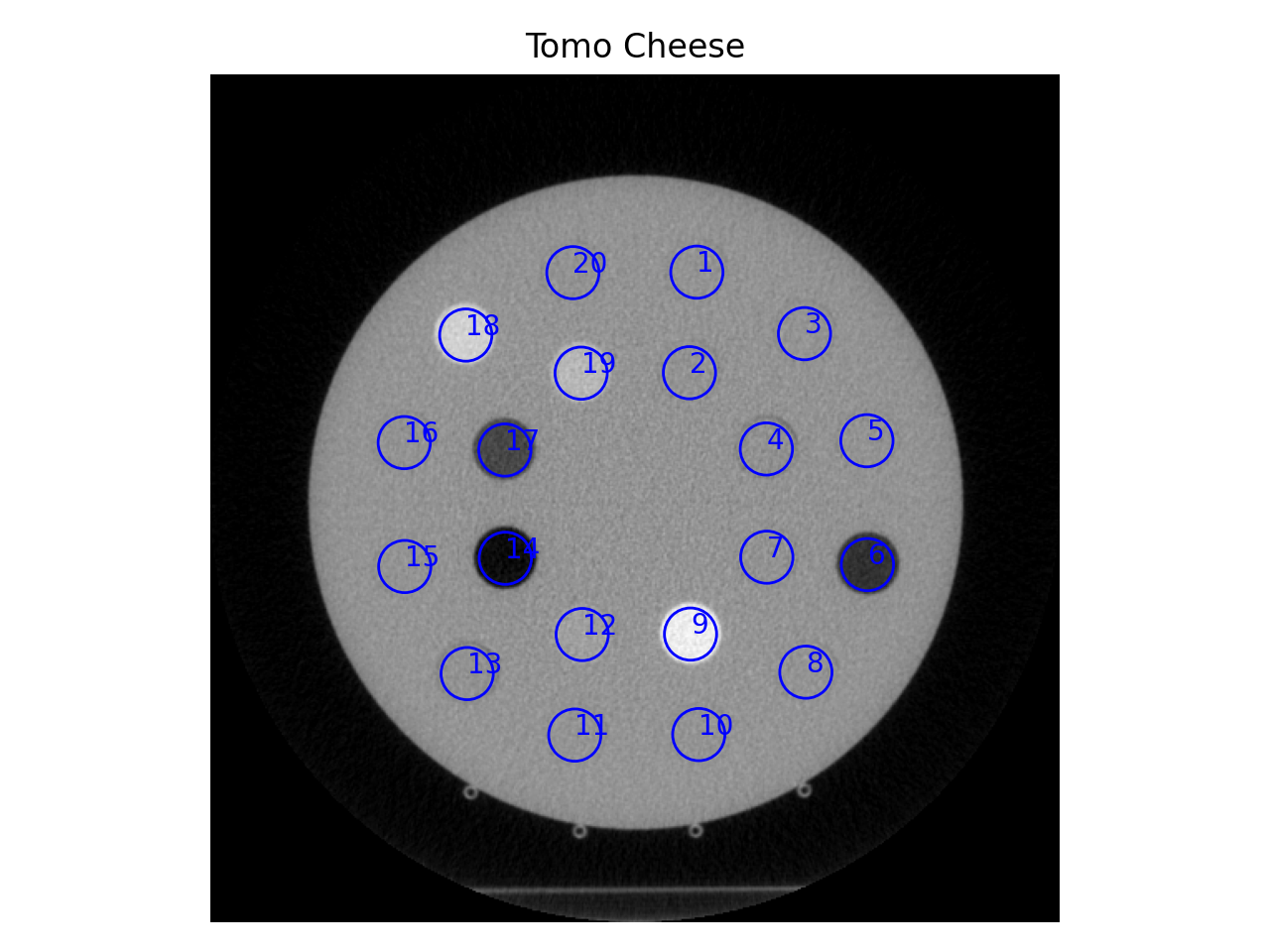
(Source code, png, hires.png, pdf)
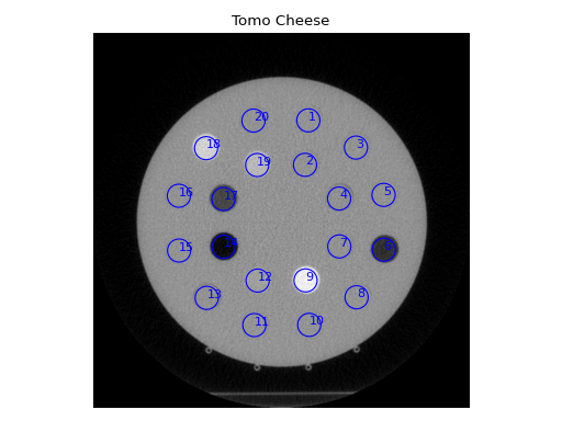
Results will be also be printed to the console:
- TomoTherapy Cheese Phantom Analysis -
- HU Module -
ROI 1 median: 17.0, stdev: 37.9
ROI 2 median: 20.0, stdev: 44.2
ROI 3 median: 23.0, stdev: 36.9
ROI 4 median: 1.0, stdev: 45.7
ROI 5 median: 17.0, stdev: 37.6
ROI 6 median: -669.0, stdev: 39.6
ROI 7 median: 14.5, stdev: 45.8
ROI 8 median: 26.0, stdev: 38.6
ROI 9 median: 653.0, stdev: 47.4
ROI 10 median: 25.0, stdev: 36.7
ROI 11 median: 24.0, stdev: 35.3
ROI 12 median: 102.0, stdev: 46.2
ROI 13 median: 8.0, stdev: 38.1
ROI 14 median: -930.0, stdev: 43.8
ROI 15 median: 23.0, stdev: 36.3
ROI 16 median: 15.0, stdev: 37.1
ROI 17 median: -516.0, stdev: 45.1
ROI 18 median: 448.0, stdev: 38.1
ROI 19 median: 269.0, stdev: 45.3
ROI 20 median: 15.0, stdev: 37.9
Typical Use
The cheese phantom analyses follows a similar pattern of load/analyze/output as the rest of the library. Unlike the CatPhan analysis, tolerances are not applied and comparison to known values is not the goal. There are two reasons for this: 1) The plugs are interchangable and thus the reference values are not necessarily constant. 2) Evaluation against a reference is not the end goal as described in the philosophy. Thus, measured values are provided; what you do with them is your business.
To use the Tomo Cheese analysis, import the class:
from pylinac import TomoCheese
And then load, analyze, and view the results:
Load images – Loading can be done with a directory or zip file:
cheese_folder = r"C:/TomoTherapy/QA/September"
cheese = TomoCheese(cheese_folder)
or load from zip:
cheese_zip = r"C:/TomoTherapy/QA/September.zip"
cheese = TomoCheese.from_zip(cheese_zip)
Analyze – Analyze the dataset:
cheese.analyze()
View the results – Reviewing the results can be done in text or dictionary format as well as images:
# print text to the console
print(cheese.results())
# return a dictionary or dataclass
results = cheese.results_data()
# view analyzed image summary
cheese.plot_analyzed_image()
# save the images
cheese.save_analyzed_image()
# finally, save a PDF
cheese.publish_pdf()
Algorithm
The TomoCheese algorithm leverages a lot of infrastructure from the CatPhan algorithm. It is not based on a manual.
Allowances
- The images can be any size.
- The phantom can have significant translation in all 3 directions.
- The phantom can have significant roll and moderate yaw and pitch.
Restrictions
Warning
Analysis can fail or give unreliable results if any Restriction is violated.
The phantom cannot touch any edge of the FOV.
There must be at least one ROI in the “outer” ROI ring that is higher than water/background phantom. This has to do with the automatic roll compensation.
Note
This is not strictly required but will assist in accurate sub-degree roll compensation.
Pre-Analysis
The pre-analysis is almost exactly the same as the CatPhan pre-analysis.
Analysis
- Determine image properties – Automatic roll compensation is attempted by creating a circular profile at the radius of the “outer” ROIs. This profile is then searched for peaks, which correspond to high-density plugs that have been inserted. If a peak is not found, no correction is applied and the phantom is assumed to be at 0. This would occur if all plugs have been filled with water/background plugs. If a peak is found, i.e. a plug has been inserted with HU detectably above water, the center of the peak is determined which would correspond to the center of the ROI. The distance to the nearest nominal ROI is calculated. If the value is <5 degrees, the roll compensation is applied. If the value is >5 degrees, the compensation is not applied and the phantom is assumed to be at 0.
- Measure HU values of each plug – Based on the nominal spacing and roll compensation (if applied), each plug area is sampled for the median and standard deviation values.
API Documentation
-
class
pylinac.cheese.TomoCheese(folderpath: Union[str, Sequence[str], pathlib.Path, Sequence[pathlib.Path], Sequence[_io.BytesIO]], check_uid: bool = True)[source]¶ Bases:
pylinac.ct.CatPhanBaseA class for analyzing the TomoTherapy ‘Cheese’ Phantom containing insert holes and plugs for HU analysis.
Parameters: - folderpath (str, list of strings, or Path to folder) – String that points to the CBCT image folder location.
- check_uid (bool) – Whether to enforce raising an error if more than one UID is found in the dataset.
Raises: NotADirectoryError– If folder str passed is not a valid directory.FileNotFoundError– If no CT images are found in the folder
-
analyze() → None[source]¶ Analyze the Tomo Cheese phantom. No parameters as the configuration isn’t known a priori
-
find_phantom_roll(func: Optional[Callable] = None) → float[source]¶ Examine the phantom for the maximum HU delta insert position. Roll the phantom by the measured angle to the nearest nominal angle if nearby. If not nearby, default to 0
-
plot_analyzed_image(show: bool = True, **plt_kwargs) → None[source]¶ Plot the images used in the calculation and summary data.
Parameters: - show (bool) – Whether to plot the image or not.
- plt_kwargs (dict) – Keyword args passed to the plt.figure() method. Allows one to set things like figure size.
-
results(as_list: bool = False) → Union[str, list][source]¶ Return the results of the analysis as a string. Use with print().
Parameters: as_list (bool) – Whether to return as a list of strings vs single string. Pretty much for internal usage.
-
results_data(as_dict: bool = False) → Union[pylinac.cheese.TomoCheeseResult, dict][source]¶ Return the results of the analysis as a structure dataclass
-
publish_pdf(filename: Union[str, pathlib.Path], notes: Optional[str] = None, open_file: bool = False, metadata: Optional[dict] = None, logo: Union[pathlib.Path, str, None] = None) → None[source]¶ Publish (print) a PDF containing the analysis and quantitative results.
Parameters: - filename ((str, file-like object}) – The file to write the results to.
- notes (str, list of strings) – Text; if str, prints single line. If list of strings, each list item is printed on its own line.
- open_file (bool) – Whether to open the file using the default program after creation.
- metadata (dict) – Extra data to be passed and shown in the PDF. The key and value will be shown with a colon. E.g. passing {‘Author’: ‘James’, ‘Unit’: ‘TrueBeam’} would result in text in the PDF like: ————– Author: James Unit: TrueBeam ————–
- logo (Path, str) – A custom logo to use in the PDF report. If nothing is passed, the default pylinac logo is used.
-
save_analyzed_subimage() → None[source]¶ Save a component image to file.
Parameters: - filename (str, file object) – The file to write the image to.
- subimage (str) – See
plot_analyzed_subimage()for parameter info. - delta (bool) – Only for use with
lin. Whether to plot the HU delta or actual values.
-
plot_analyzed_subimage() → None[source]¶ Plot a specific component of the CBCT analysis.
Parameters: - subimage ({'hu', 'un', 'sp', 'lc', 'mtf', 'lin', 'prof'}) –
The subcomponent to plot. Values must contain one of the following letter combinations. E.g.
linearity,linear, andlinwill all draw the HU linearity values.hudraws the HU linearity image.undraws the HU uniformity image.spdraws the Spatial Resolution image.lcdraws the Low Contrast image (if applicable).mtfdraws the RMTF plot.lindraws the HU linearity values. Used withdelta.profdraws the HU uniformity profiles.
- delta (bool) – Only for use with
lin. Whether to plot the HU delta or actual values. - show (bool) – Whether to actually show the plot.
- subimage ({'hu', 'un', 'sp', 'lc', 'mtf', 'lin', 'prof'}) –
-
catphan_size¶ The expected size of the phantom in pixels, based on a 20cm wide phantom.
-
find_origin_slice() → int¶ Using a brute force search of the images, find the median HU linearity slice.
This method walks through all the images and takes a collapsed circle profile where the HU linearity ROIs are. If the profile contains both low (<800) and high (>800) HU values and most values are the same (i.e. it’s not an artifact), then it can be assumed it is an HU linearity slice. The median of all applicable slices is the center of the HU slice.
Returns: The middle slice of the HU linearity module. Return type: int
-
find_phantom_axis() -> (typing.Callable, typing.Callable)¶ We fit all the center locations of the phantom across all slices to a 1D poly function instead of finding them individually for robustness.
Normally, each slice would be evaluated individually, but the RadMachine jig gets in the way of detecting the HU module (🤦♂️). To work around that in a backwards-compatible way we instead look at all the slices and if the phantom was detected, capture the phantom center. ALL the centers are then fitted to a 1D poly function and passed to the individual slices. This way, even if one slice is messed up (such as because of the phantom jig), the poly function is robust to give the real center based on all the other properly-located positions on the other slices.
-
classmethod
from_demo_images()¶ Construct a CBCT object from the demo images.
-
classmethod
from_url(url: str, check_uid: bool = True)¶ Instantiate a CBCT object from a URL pointing to a .zip object.
Parameters: - url (str) – URL pointing to a zip archive of CBCT images.
- check_uid (bool) – Whether to enforce raising an error if more than one UID is found in the dataset.
-
classmethod
from_zip(zip_file: Union[str, zipfile.ZipFile, BinaryIO], check_uid: bool = True)¶ Construct a CBCT object and pass the zip file.
Parameters: - zip_file (str, ZipFile) – Path to the zip file or a ZipFile object.
- check_uid (bool) – Whether to enforce raising an error if more than one UID is found in the dataset.
Raises: - FileExistsError : If zip_file passed was not a legitimate zip file.
- FileNotFoundError : If no CT images are found in the folder
-
localize() → None¶ Find the slice number of the catphan’s HU linearity module and roll angle
-
mm_per_pixel¶ The millimeters per pixel of the DICOM images.
-
num_images¶ The number of images loaded.
-
save_analyzed_image(filename: Union[str, pathlib.Path, BinaryIO], **kwargs) → None¶ Save the analyzed summary plot.
Parameters: - filename (str, file object) – The name of the file to save the image to.
- kwargs – Any valid matplotlib kwargs.
-
class
pylinac.cheese.TomoCheeseModule(catphan, tolerance: Optional[float] = None, offset: int = 0, clear_borders: bool = True)[source]¶ Bases:
pylinac.ct.CatPhanModuleThe pluggable module with user-accessible holes.
The ROIs of the inner circle are ~45 degrees apart. The ROIs of the outer circle are ~30 degrees apart
-
plot_rois(axis: matplotlib.axes._axes.Axes) → None[source]¶ Plot the ROIs to the axis. We add the ROI # to help the user differentiate
-
is_phantom_in_view() → bool¶ Whether the phantom appears to be within the slice.
-
phan_center¶ Determine the location of the center of the phantom.
-
phantom_roi¶ Get the Scikit-Image ROI of the phantom
The image is analyzed to see if: 1) the CatPhan is even in the image (if there were any ROIs detected) 2) an ROI is within the size criteria of the catphan 3) the ROI area that is filled compared to the bounding box area is close to that of a circle
-
plot(axis: matplotlib.axes._axes.Axes)¶ Plot the image along with ROIs to an axis
-
preprocess(catphan)¶ A preprocessing step before analyzing the CTP module.
Parameters: catphan (~pylinac.cbct.CatPhanBase instance.) –
-
roi_dist_mm¶ alias of
builtins.float
-
slice_num¶ The slice number of the spatial resolution module.
Returns: Return type: float
-
-
class
pylinac.cheese.TomoCheeseResult(origin_slice: int, num_images: int, phantom_roll: float, roi_1: dict, roi_2: dict, roi_3: dict, roi_4: dict, roi_5: dict, roi_6: dict, roi_7: dict, roi_8: dict, roi_9: dict, roi_10: dict, roi_11: dict, roi_12: dict, roi_13: dict, roi_14: dict, roi_15: dict, roi_16: dict, roi_17: dict, roi_18: dict, roi_19: dict, roi_20: dict)[source]¶ Bases:
pylinac.core.utilities.ResultBaseThis class should not be called directly. It is returned by the
results_data()method. It is a dataclass under the hood and thus comes with all the dunder magic.Use the following attributes as normal class attributes.
-
origin_slice= None
-
num_images= None
-
phantom_roll= None
-
roi_1= None
-
roi_2= None
-
roi_3= None
-
roi_4= None
-
roi_5= None
-
roi_6= None
-
roi_7= None
-
roi_8= None
-
roi_9= None
-
roi_10= None
-
roi_11= None
-
roi_12= None
-
roi_13= None
-
roi_14= None
-
roi_15= None
-
roi_16= None
-
roi_17= None
-
roi_18= None
-
roi_19= None
-
roi_20= None
-