ACR Phantoms
Overview
Added in version 3.2.
Warning
These algorithms have only a limited amount of testing data and results should be scrutinized. Further, the algorithm is more likely to change in the future when a more robust test suite is built up. If you’d like to submit data, enter it here.
The ACR module provides routines for automatically analyzing DICOM images of the ACR CT 464 phantom and Large MR phantom. It can load a folder or zip file of images, correcting for translational and rotational offsets.
Phantom reference information is drawn from the ACR CT solution article and the analysis is drawn from the ACR CT testing article. MR analysis is drawn from the ACR Guidance document.
Warning
Due to the rectangular ROIs on the MRI phantom analysis, rotational errors should be <= 1 degree. Translational errors are still accounted for however for any reasonable amount.
Typical Use
The ACR CT and MR analyses follows a similar pattern of load/analyze/output as the rest of the library. Unlike the CatPhan analysis, customization is not a goal, as the phantoms and analyses are much more well-defined. I.e. there’s less of a use case for custom phantoms in this scenario. CT is mostly used here but is interchangeable with the MRI class.
To use the ACR analysis, import the class:
from pylinac import ACRCT, ACRMRILarge
And then load, analyze, and view the results:
Load images – Loading can be done with a directory or zip file:
acr_ct_folder = r"C:/CT/ACR/Sept 2021"
ct = ACRCT(acr_ct_folder)
acr_mri_folder = r"C:/MRI/ACR/Sept 2021"
mri = ACRMRILarge(acr_mri_folder)
or load from zip:
acr_ct_zip = r"C:/CT/ACR/Sept 2021.zip"
ct = ACRCT.from_zip(acr_ct_zip)
Analyze – Analyze the dataset:
ct.analyze()
View the results – Reviewing the results can be done in text or dict format as well as images:
# print text to the console
print(ct.results())
# view analyzed image summary
ct.plot_analyzed_image()
# view images independently
ct.plot_images()
# save the images
ct.save_analyzed_image()
# or
ct.save_images()
# finally, save a PDF
ct.publish_pdf()
Choosing an MR Echo
With MRI, a dual echo scan can be obtained. These can result in a combined DICOM dataset but are distinct
acquisitions. To select between multiple echos, use the echo_number parameter:
from pylinac import ACRMRILarge

mri = ACRMRILarge(...)  # load zip or dir with dual echo image set
mri.analyze(echo_number=2)
mri.results()
If no echo number is passed, the first and lowest echo number is selected and analyzed.
Customizing MR/CT Modules
To customize aspects of the MR analysis modules, subclass the relevant module and set the attribute in the analysis class. E.g. to customize the “Slice1” MR module:
from pylinac.acr import ACRMRILarge, MRSlice1Module


class Slice1Modified(MRSlice1Module):
    """Custom location for the slice thickness ROIs"""

    thickness_roi_settings = {
        "Top": {"width": 100, "height": 4, "distance": -3},
        "Bottom": {"width": 100, "height": 4, "distance": 2.5},
    }


# now pass to the MR analysis class
class MyMRI(ACRMRILarge):
    slice1 = Slice1Modified


# use as normal
mri = MyMRI(...)
mri.analyze(...)
There are 4 modules in ACR MRI Large analysis that can be overridden. The attribute name should stay the same but the name of the subclassed module can be anything as long as it subclasses the original module:
class ACRMRILarge:
    # overload these as you wish. The attribute name cannot change.
    slice1 = MRSlice1Module
    geometric_distortion = GeometricDistortionModule
    uniformity_module = MRUniformityModule
    slice11 = MRSlice11PositionModule


class ACRCT:
    ct_calibration_module = CTModule
    low_contrast_module = LowContrastModule
    spatial_resolution_module = SpatialResolutionModule
    uniformity_module = UniformityModule
Customizing module offsets
Customizing the module offsets in the ACR module is easier than for the CT module. To do so, simply override any relevant constant like so:
import pylinac

pylinac.acr.MR_SLICE11_MODULE_OFFSET_MM = 95

mri = pylinac.ACRMRILarge(...)  # will use offset above
The options for module offsets are as follows along with their default value:
# CT
CT_UNIFORMITY_MODULE_OFFSET_MM = 70
CT_SPATIAL_RESOLUTION_MODULE_OFFSET_MM = 100
CT_LOW_CONTRAST_MODULE_OFFSET_MM = 30

# MR
MR_SLICE11_MODULE_OFFSET_MM = 100
MR_GEOMETRIC_DISTORTION_MODULE_OFFSET_MM = 40
MR_UNIFORMITY_MODULE_OFFSET_MM = 60
Advanced Use
Using results_data
Using the ACR module in your own scripts? While the analysis results can be printed out,
if you intend on using them elsewhere (e.g. in an API), they can be accessed the easiest by using the results_data() method
which returns a ACRCTResult instance. For MRI this is results_data() method
and ACRMRIResult respectively.
Continuing from above:
data = ct.results_data()
data.ct_module.roi_radius_mm
# and more

# return as a dict
data_dict = ct.results_data(as_dict=True)
data_dict["ct_module"]["roi_radius_mm"]
...
CT Analysis Parameters
See pylinac.acr.ACRCT.analyze() for details.
There are currently no analysis parameters for the ACR CT phantom.
Interpreting CT Results
The outcome from analyzing the phantom and calling .results_data() is a ACRCTResult instance.
See the API documentation for details and also Exporting Results.
The outcome from analyzing the phantom in RadMachine will return an “Entire Result” as follows:
phantom_model: The model of the phantom used.phantom_roll_deg: The roll of the phantom in degrees.origin_slice: The slice number of the “origin” slice; for ACR this is Module 1.num_images: The number of images in the passed dataset.ct_module: The results of the CT module with the following items:offset: The offset of the module slice in mm from the origin slice (z-direction).roi_distance_from_center_mm: The distance of the ROIs from the center of the phantom in mm in the image plane.roi_radius_mm: The radius of the ROIs in mm.rois: The analyzed ROIs. The key is the name of the material and the value is the mean HU value. E.g.'Air': -987.1.roi_settings: The ROI settings. The keys are the material names, each with the following items:angle: The angle of the ROI in degrees.distance: The distance of the ROI from the center of the phantom in mm.radius: The radius of the ROI in mm.distance_pixels: The distance of the ROI from the center of the phantom in pixels.radius_pixels: The radius of the ROI in pixels.angle_corrected: The angle of the ROI corrected for phantom roll in degrees.
uniformity_module: The results from the Uniformity module, with the following items:offset: The offset of the module slice in mm from the origin slice (z-direction).roi_distance_from_center_mm: The distance of the ROIs from the center of the phantom in mm in the image plane.roi_radius_mm: The radius of the ROIs in mm.rois: The analyzed ROIs. The key is the location and the value is the mean HU value. E.g.'Top': 13.2.roi_settings: The ROI settings. The keys are the location names.center_roi_stdev: The standard deviation of the center ROI.
low_contrast_module: The results of the Low-Contrast module, with the following items:offset: The offset of the module slice in mm from the origin slice (z-direction).roi_distance_from_center_mm: The distance of the ROIs from the center of the phantom in mm in the image plane.roi_radius_mm: The radius of the ROIs in mm.rois: The analyzed ROI values.roi_settings: The ROI settings.cnr: The contrast-to-noise ratio.
spatial_resolution_module: The results of the Spatial Resolution module, with the following items:offset: The offset of the module slice in mm from the origin slice (z-direction).roi_distance_from_center_mm: The distance of the ROIs from the center of the phantom in mm in the image plane.roi_radius_mm: The radius of the ROIs in mm.rois: The analyzed ROIs. The key is the location and the value is the mean HU value. E.g.'Top': 13.2.roi_settings: The ROI settings. The keys are the location names.lpmm_to_rmtf: Line pair to relative modulation transfer mapping. The keys are the line pair values and the values are the relative modulation transfer values.
MRI Algorithm
The ACR MR analysis is based on the official guidance document. Because the guidance document is extremely specific (nice job ACR!) only a few highlights are given here. The guidance is followed as reasonably close as possible.
Allowances
Multiple MR sequences can be present in the dataset.
The phantom can have significant cartesian shifts.
Restrictions
There should be 11 slices per scan (although multiple echo scans are allowed) per the guidance document (section 0.3).
The phantom should have very little pitch, yaw, or roll (<1 degree).
Troubleshooting
The MRI phantom specifically can suffer from evaporation of the water in the phantom. This causes bubbles to appear physically and also creates artifacts in the image. Large enough air in the phantom can cause an analysis to fail and/or create shifting issues in the analysis.
If bubbles are present, you can send it to the manufacturer to be fixed, or you can fill it yourself per this YouTube video: Filling the ACR MRI Phantom.
Analysis
Section 0.4 specifies the 7 tests to perform. Pylinac can perform 6 of these 7. It cannot yet perform the low-contrast visibility test.
Geometric Accuracy - The geometric accuracy is measured using profiles of slice 5. The only difference is that pylinac will use the 60th percentile pixel value of the image as a high-pass filter so that minor background fluctuations are removed and then take the FWHM of several profiles of this new image. The width between the two pixels defining the FWHM is the diameter.
High Contrast - High contrast is hard to measure for the ACR MRI phantom simply because it does not use line pairs, but rather offset dots as well as the qualitative description in the guidance document about how to score these. Pylinac measures the high-contrast by sampling a circular ROI on the left ROI (phantom right) set. This is the baseline which all other measurements will be normalized to. The actual dot-ROIs are sampled by taking a circular ROI of the row-based set and the column-based set. Each row-based ROI is evaluated against the other row-based ROIs. The same is done for column-based ROIs. The ROIs use the maximum and minimum pixel values inside the sample ROI. No dot-counting is performed.
Tip
It is suggested to perform the contrast measurement visually and compare to pylinac values to establish a cross-comparison ratio. After a ratio has been established, the pylinac MTF can be used as the baseline value moving forward.
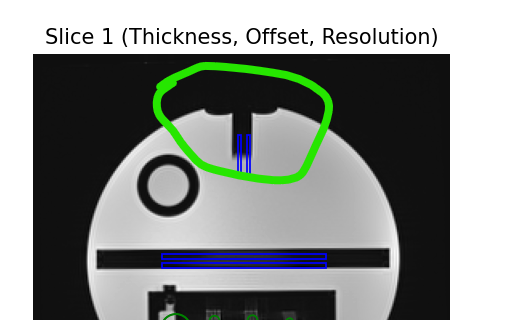
Slice thickness - Slice thickness is measured using the FWHM of two rectangular ROIs. This is very similar to the guidance document explanation.
Slice thickness is defined the same as in the guidance document:
\[Thickness = 0.2 * \frac{Top * Bottom}{Top + Bottom}\]Slice Position - Slice position accuracy is measured very similarly to the manual method described in the document: “The display level setting … should be set to a level roughly half that of the signal in the bright, all-water portions of the phantom.” For each vertical bar, the pixel nearest to the mid-value between min and max of the rectangular ROI is used as the bar position:
\[position_{bar} = \frac{ROI_{max} - ROI_{min}}{2} + ROI_{min}\]The difference in positions between the bars is the value reported.
Uniformity - Uniformity is measured using a circular ROI at the center of the phantom and ROIs to the top, bottom, left, and right of the phantom, very similar to the guidance document.
The percent integral uniformity (PIU) is defined as:
\[PIU = 100 * (1 - \frac{high-low}{high+low})\]Instead of using the WL/WW to find the low and high 1cm2 ROI, pylinac uses the 1st and 99th percentile of pixel values inside the central ROI.
The ghosting ratio is defined the same as the ACR guidance document:
\[ghosting_{ratio} = |\frac{(top + bottom) - (left + right)}{2*ROI_{large}}|\]where all values are the median pixel values of their respective ROI. The percent-signal ghosting (PSG) is:
\[PSG = ghosting_{ratio} * 100\]
MRI Analysis Parameters
See pylinac.acr.ACRMRILarge.analyze() for details.
Echo Number: The echo sequence to analyze; uses the Echo Numbers DICOM tag. Only relevant if more than one echo sequence is present in the dataset. If multiple echos are detected, the default is to analyze the first echo sequence.
Interpreting MRI Results
The outcome from analyzing the phantom and calling .results_data() is a ACRMRIResult instance.
See the API documentation for details and also Exporting Results.
The outcome from analyzing the phantom in RadMachine will return an “Entire Result” as follows:
phantom_model: The model of the phantom used.phantom_roll_deg: The roll of the phantom in degrees.origin_slice: The slice number of the “origin” slice; for ACR this is Slice 1.num_images: The number of images in the passed dataset.slice1: The results for the “Slice 1” module with the following items:offset: The offset of the phantom in mm from the origin slice.bar_difference_mm: The difference in bar positions in mm.slice_shift_mm: The measured shift in slice position compared to nominal.measured_slice_thickness_mm: The measured slice thickness in mm.row_mtf_50: The MTF at 50% for the row-based ROIs.col_mtf_50: The MTF at 50% for the column-based ROIs.rois: A dictionary of the analyzed MTF ROIs. The key is the name of the ROI; e.g.Row 1.1and the key is a dictionary of the following items:name: The name of the ROI.value: The mean HU value of the ROI.stdev: The standard deviation of the ROI.
roi_settings: A dictionary of the ROI settings. The keys are the ROI names, each with the following items:angle: The angle of the ROI in degrees.distance: The distance of the ROI from the center of the phantom in mm.radius: The radius of the ROI in mm.distance_pixels: The distance of the ROI from the center of the phantom in pixels.radius_pixels: The radius of the ROI in pixels.angle_corrected: The angle of the ROI corrected for phantom roll in degrees.
slice11: A dictionary of results from the analysis of “Slice 11” with the ‘ following items:offset: The offset of the phantom in mm from the origin slice.bar_difference_mm: The difference in bar positions in mm.slice_shift_mm: The measure shift in slice position compared to nominal.rois: The results of the left and right bar ROIs. The key is the name of the bar and the results are a dictionary with the following items:name: The name of the ROI.value: The mean HU value of the ROI.stdev: The standard deviation of the ROI.roi_settings: The ROI settings. The keys are the ROI names, each with the following items:angle: The angle of the ROI in degrees.distance: The distance of the ROI from the center of the phantom in mm.radius: The radius of the ROI in mm.distance_pixels: The distance of the ROI from the center of the phantom in pixels.radius_pixels: The radius of the ROI in pixels.angle_corrected: The angle of the ROI corrected for phantom roll in degrees.
uniformity_module: Results from the uniformity module with the following items:offset: The offset of the phantom in mm from the origin slice.ghosting_ratio: The ghosting ratio.piu: The percent integral uniformity.piu_passed: Whether the PIU passed the test.psg: The percent signal ghosting.rois: A dictionary of the analyzed ROIs. The key is the name of the ROI region with the following items:name: The name of the ROI.value: The mean HU value of the ROI.stdev: The standard deviation of the ROI.difference: The difference in HU value from the nominal value.nominal_value: The nominal HU value of the ROI.passed: Whether the ROI passed the test.
roi_settings: A dictionary of the ROI settings. The keys are the ROI names, each with the following items:angle: The angle of the ROI in degrees.distance: The distance of the ROI from the center of the phantom in mm.radius: The radius of the ROI in mm.distance_pixels: The distance of the ROI from the center of the phantom in pixels.radius_pixels: The radius of the ROI in pixels.angle_corrected: The angle of the ROI corrected for phantom roll in degrees.
ghost_rois: A dictionary of the analyzed ghosting ROIs. The key is the name of the ROI region with the following items:name: The name of the ROI.value: The mean HU value of the ROI.stdev: The standard deviation of the ROI.
ghost_roi_settings: A dictionary of the ghosting ROI settings. The keys are the ROI names, each with the following items:angle: The angle of the ROI in degrees.distance: The distance of the ROI from the center of the phantom in mm.radius: The radius of the ROI in mm.distance_pixels: The distance of the ROI from the center of the phantom in pixels.radius_pixels: The radius of the ROI in pixels.angle_corrected: The angle of the ROI corrected for phantom roll in degrees.
geometric_distortion_module: Results from the geometric distortion module with the following items:offset: The offset of the phantom in mm from the origin slice.profiles: A dictionary of the profiles used to measure the geometric distortion. The key is the name of the profile and the value is a dictionary with the following items:width_mm: The FWHM of the profile in mm.line: A dictionary representing the line to be plotted.
distances: The lines measuring the ROI size. The key is the name of the line direction and the value is a string of the line length.
API Documentation
- class pylinac.acr.ACRCT(folderpath: str | Sequence[str] | Path | Sequence[Path] | Sequence[BytesIO], check_uid: bool = True, memory_efficient_mode: bool = False)[source]
Bases:
CatPhanBase,ResultsDataMixin[ACRCTResult]Parameters
- folderpathstr, list of strings, or Path to folder
String that points to the CBCT image folder location.
- check_uidbool
Whether to enforce raising an error if more than one UID is found in the dataset.
- memory_efficient_modebool
Whether to use a memory efficient mode. If True, the DICOM stack will be loaded on demand rather than all at once. This will reduce the memory footprint but will be slower by ~25%. Default is False.
Raises
- NotADirectoryError
If folder str passed is not a valid directory.
- FileNotFoundError
If no CT images are found in the folder
- ct_calibration_module
alias of
CTModule
- low_contrast_module
alias of
LowContrastModule
- spatial_resolution_module
alias of
SpatialResolutionModule
- uniformity_module
alias of
UniformityModule
- plot_analyzed_subimage(*args, **kwargs)[source]
Plot a specific component of the CBCT analysis.
Parameters
- subimage{‘hu’, ‘un’, ‘sp’, ‘lc’, ‘mtf’, ‘lin’, ‘prof’, ‘side’}
The subcomponent to plot. Values must contain one of the following letter combinations. E.g.
linearity,linear, andlinwill all draw the HU linearity values.hudraws the HU linearity image.undraws the HU uniformity image.spdraws the Spatial Resolution image.lcdraws the Low Contrast image (if applicable).mtfdraws the RMTF plot.lindraws the HU linearity values. Used withdelta.profdraws the HU uniformity profiles.sidedraws the side view of the phantom with lines of the module locations.
- deltabool
Only for use with
lin. Whether to plot the HU delta or actual values.- showbool
Whether to actually show the plot.
- save_analyzed_subimage(*args, **kwargs)[source]
Save a component image to file.
Parameters
- filenamestr, file object
The file to write the image to.
- subimagestr
See
plot_analyzed_subimage()for parameter info.- deltabool
Only for use with
lin. Whether to plot the HU delta or actual values.
- plotly_analyzed_image(show: bool = True, show_colorbar: bool = True, show_legend: bool = True, **kwargs) dict[str, Figure][source]
Plot the analyzed image using Plotly. Will create multiple figures.
Parameters
- showbool
Whether to show the images. Set to False if doing further processing of the figure.
- show_colorbarbool
Whether to show the colorbar on the images.
- show_legendbool
Whether to show the legend on the images.
- kwargs
Additional keyword arguments to pass to the figure.
- plot_analyzed_image(show: bool = True, **plt_kwargs) Figure[source]
Plot the analyzed image
Parameters
- show
Whether to show the image.
- plt_kwargs
Keywords to pass to matplotlib for figure customization.
- save_analyzed_image(filename: str | Path | BytesIO, **plt_kwargs) None[source]
Save the analyzed image to disk or stream
Parameters
- filename
Where to save the image to
- plt_kwargs
Keywords to pass to matplotlib for figure customization.
- plot_images(show: bool = True, **plt_kwargs) dict[str, Figure][source]
Plot all the individual images separately
Parameters
- show
Whether to show the images.
- plt_kwargs
Keywords to pass to matplotlib for figure customization.
- save_images(directory: Path | str | None = None, to_stream: bool = False, **plt_kwargs) list[Path | BytesIO][source]
Save separate images to disk or stream.
Parameters
- directory
The directory to write the images to. If None, will use current working directory
- to_stream
Whether to write to stream or disk. If True, will return streams. Directory is ignored in that scenario.
- plt_kwargs
Keywords to pass to matplotlib for figure customization.
- find_phantom_roll(func=<function ACRCT.<lambda>>) float[source]
Determine the “roll” of the phantom.
Only difference of base method is that we sort the ROIs by size, not by being in the center since the two we’re looking for are both right-sided.
- publish_pdf(filename: str | Path, notes: str | None = None, open_file: bool = False, metadata: dict | None = None, logo: Path | str | None = None) None[source]
Publish (print) a PDF containing the analysis and quantitative results.
Parameters
- filename(str, file-like object}
The file to write the results to.
- notesstr, list of strings
Text; if str, prints single line. If list of strings, each list item is printed on its own line.
- open_filebool
Whether to open the file using the default program after creation.
- metadatadict
Extra data to be passed and shown in the PDF. The key and value will be shown with a colon. E.g. passing {‘Author’: ‘James’, ‘Unit’: ‘TrueBeam’} would result in text in the PDF like: ————– Author: James Unit: TrueBeam ————–
- logo: Path, str
A custom logo to use in the PDF report. If nothing is passed, the default pylinac logo is used.
- property catphan_size: float
The expected size of the phantom in pixels, based on a 20cm wide phantom.
- find_origin_slice() int
Using a brute force search of the images, find the median HU linearity slice.
This method walks through all the images and takes a collapsed circle profile where the HU linearity ROIs are. If the profile contains both low (<800) and high (>800) HU values and most values are the same (i.e. it’s not an artifact), then it can be assumed it is an HU linearity slice. The median of all applicable slices is the center of the HU slice.
Returns
- int
The middle slice of the HU linearity module.
- find_phantom_axis()
We fit all the center locations of the phantom across all slices to a 1D poly function instead of finding them individually for robustness.
Normally, each slice would be evaluated individually, but the RadMachine jig gets in the way of detecting the HU module (🤦♂️). To work around that in a backwards-compatible way we instead look at all the slices and if the phantom was detected, capture the phantom center. ALL the centers are then fitted to a 1D poly function and passed to the individual slices. This way, even if one slice is messed up (such as because of the phantom jig), the poly function is robust to give the real center based on all the other properly-located positions on the other slices.
- classmethod from_demo_images()
Construct a CBCT object from the demo images.
- classmethod from_url(url: str, check_uid: bool = True)
Instantiate a CBCT object from a URL pointing to a .zip object.
Parameters
- urlstr
URL pointing to a zip archive of CBCT images.
- check_uidbool
Whether to enforce raising an error if more than one UID is found in the dataset.
- classmethod from_zip(zip_file: str | ZipFile | BinaryIO, check_uid: bool = True, memory_efficient_mode: bool = False)
Construct a CBCT object and pass the zip file.
Parameters
- zip_filestr, ZipFile
Path to the zip file or a ZipFile object.
- check_uidbool
Whether to enforce raising an error if more than one UID is found in the dataset.
- memory_efficient_modebool
Whether to use a memory efficient mode. If True, the DICOM stack will be loaded on demand rather than all at once. This will reduce the memory footprint but will be slower by ~25%. Default is False.
Raises
FileExistsError : If zip_file passed was not a legitimate zip file. FileNotFoundError : If no CT images are found in the folder
- localize() None
Find the slice number of the catphan’s HU linearity module and roll angle
- property mm_per_pixel: float
The millimeters per pixel of the DICOM images.
- property num_images: int
The number of images loaded.
- plot_side_view(axis: Axes) None
Plot a view of the scan from the side with lines showing detected module positions
- refine_origin_slice(initial_slice_num: int) int
Apply a refinement to the origin slice. This was added to handle the catphan 604 at least due to variations in the length of the HU plugs.
- results_data(as_dict: bool = False, as_json: bool = False, by_alias: bool = False, exclude: set[str] | None = None) T | dict | str
Present the results data and metadata as a dataclass, dict, or tuple. The default return type is a dataclass.
Parameters
- as_dictbool
If True, return the results as a dictionary.
- as_jsonbool
If True, return the results as a JSON string. Cannot be True if as_dict is True.
- by_aliasbool
If True, use the alias names of the dataclass fields. These are generally the more human-readable names.
- excludeset
A set of fields to exclude from the results data.
- to_quaac(path: str | Path, performer: User, primary_equipment: Equipment, format: Literal['json', 'yaml'] = 'yaml', attachments: list[Attachment] | None = None, overwrite: bool = False, **kwargs) None
Write an analysis to a QuAAC file. This will include the items from results_data() and the PDF report.
Parameters
- pathstr, Path
The file to write the results to.
- performerUser
The user who performed the analysis.
- primary_equipmentEquipment
The equipment used in the analysis.
- format{‘json’, ‘yaml’}
The format to write the file in.
- attachmentslist of Attachment
Additional attachments to include in the QuAAC file.
- overwritebool
Whether to overwrite the file if it already exists.
- kwargs
Additional keyword arguments to pass to the Document instantiation.
- pydantic model pylinac.acr.ACRCTResult[source]
Bases:
ResultBaseThis class should not be called directly. It is returned by the
results_data()method.Use the following attributes as normal class attributes.
Create a new model by parsing and validating input data from keyword arguments.
Raises [ValidationError][pydantic_core.ValidationError] if the input data cannot be validated to form a valid model.
self is explicitly positional-only to allow self as a field name.
- field phantom_model: str [Required]
The model of the phantom used.
- field phantom_roll_deg: float [Required]
The roll of the phantom in degrees.
- field origin_slice: int [Required]
The slice number of the ‘origin’ slice; for ACR this is Module 1.
- field num_images: int [Required]
The number of images in the passed dataset.
- field ct_module: CTModuleOutput [Required]
The results of the CT module.
- field uniformity_module: UniformityModuleOutput [Required]
The results of the Uniformity module.
- field low_contrast_module: LowContrastModuleOutput [Required]
The results of the Low Contrast module.
- field spatial_resolution_module: SpatialResolutionModuleOutput [Required]
The results of the Spatial Resolution module.
- pydantic model pylinac.acr.CTModuleOutput[source]
Bases:
BaseModelThis class should not be called directly. It is returned by the
results_data()method.Use the following attributes as normal class attributes.
Create a new model by parsing and validating input data from keyword arguments.
Raises [ValidationError][pydantic_core.ValidationError] if the input data cannot be validated to form a valid model.
self is explicitly positional-only to allow self as a field name.
- field offset: float [Required]
The offset of the module slice in mm from the origin slice (z-direction).
- field roi_distance_from_center_mm: float [Required]
The distance of the ROIs from the center of the phantom in mm in the image plane.
- field roi_radius_mm: float [Required]
The radius of the ROIs in mm.
- field roi_settings: dict [Required]
The ROI settings. The keys are the material names.
- field rois: dict[str, float] [Required]
The analyzed ROIs. The key is the name of the material and the value is the mean HU value. E.g.
'Air': -987.1.
- pydantic model pylinac.acr.UniformityModuleOutput[source]
Bases:
CTModuleOutputThis class should not be called directly. It is returned by the
results_data()method.Use the following attributes as normal class attributes.
Create a new model by parsing and validating input data from keyword arguments.
Raises [ValidationError][pydantic_core.ValidationError] if the input data cannot be validated to form a valid model.
self is explicitly positional-only to allow self as a field name.
- field center_roi_stdev: float [Required]
The standard deviation of the center ROI.
- pydantic model pylinac.acr.SpatialResolutionModuleOutput[source]
Bases:
CTModuleOutputThis class should not be called directly. It is returned by the
results_data()method.Use the following attributes as normal class attributes.
Create a new model by parsing and validating input data from keyword arguments.
Raises [ValidationError][pydantic_core.ValidationError] if the input data cannot be validated to form a valid model.
self is explicitly positional-only to allow self as a field name.
- field lpmm_to_rmtf: dict [Required]
Line pair to relative modulation transfer mapping. The keys are the line pair values and the values are the relative modulation transfer values.
- pydantic model pylinac.acr.LowContrastModuleOutput[source]
Bases:
CTModuleOutputThis class should not be called directly. It is returned by the
results_data()method. It is a dataclass under the hood and thus comes with all the dunder magic.Use the following attributes as normal class attributes.
Create a new model by parsing and validating input data from keyword arguments.
Raises [ValidationError][pydantic_core.ValidationError] if the input data cannot be validated to form a valid model.
self is explicitly positional-only to allow self as a field name.
- field cnr: float [Required]
The contrast-to-noise ratio.
- class pylinac.acr.ACRMRILarge(folderpath: str | Sequence[str] | Path | Sequence[Path] | Sequence[BytesIO], check_uid: bool = True, memory_efficient_mode: bool = False)[source]
Bases:
CatPhanBase,ResultsDataMixin[ACRMRIResult]Parameters
- folderpathstr, list of strings, or Path to folder
String that points to the CBCT image folder location.
- check_uidbool
Whether to enforce raising an error if more than one UID is found in the dataset.
- memory_efficient_modebool
Whether to use a memory efficient mode. If True, the DICOM stack will be loaded on demand rather than all at once. This will reduce the memory footprint but will be slower by ~25%. Default is False.
Raises
- NotADirectoryError
If folder str passed is not a valid directory.
- FileNotFoundError
If no CT images are found in the folder
- slice1
alias of
MRSlice1Module
- geometric_distortion
alias of
GeometricDistortionModule
- uniformity_module
alias of
MRUniformityModule
- slice11
alias of
MRSlice11PositionModule
- plot_analyzed_subimage(*args, **kwargs)[source]
Plot a specific component of the CBCT analysis.
Parameters
- subimage{‘hu’, ‘un’, ‘sp’, ‘lc’, ‘mtf’, ‘lin’, ‘prof’, ‘side’}
The subcomponent to plot. Values must contain one of the following letter combinations. E.g.
linearity,linear, andlinwill all draw the HU linearity values.hudraws the HU linearity image.undraws the HU uniformity image.spdraws the Spatial Resolution image.lcdraws the Low Contrast image (if applicable).mtfdraws the RMTF plot.lindraws the HU linearity values. Used withdelta.profdraws the HU uniformity profiles.sidedraws the side view of the phantom with lines of the module locations.
- deltabool
Only for use with
lin. Whether to plot the HU delta or actual values.- showbool
Whether to actually show the plot.
- save_analyzed_subimage(*args, **kwargs)[source]
Save a component image to file.
Parameters
- filenamestr, file object
The file to write the image to.
- subimagestr
See
plot_analyzed_subimage()for parameter info.- deltabool
Only for use with
lin. Whether to plot the HU delta or actual values.
- find_phantom_roll() float[source]
Determine the “roll” of the phantom. This algorithm uses the circular left-upper hole on slice 1 as the reference
Returns
float : the angle of the phantom in degrees.
- analyze(echo_number: int | None = None) None[source]
Analyze the ACR CT phantom
Parameters
- echo_number:
The echo to analyze. If not passed, uses the minimum echo number found.
- plotly_analyzed_image(show: bool = True, show_colorbar: bool = True, show_legend: bool = True, **kwargs) dict[str, Figure][source]
Plot the analyzed set of images to Plotly figures.
Parameters
- showbool
Whether to show the plot.
- show_colorbarbool
Whether to show the colorbar on the plot.
- show_legendbool
Whether to show the legend on the plot.
- kwargs
Additional keyword arguments to pass to the plot.
Returns
- dict
A dictionary of the Plotly figures where the key is the name of the image and the value is the figure.
- plot_analyzed_image(show: bool = True, **plt_kwargs) Figure[source]
Plot the analyzed image
Parameters
- show
Whether to show the image.
- plt_kwargs
Keywords to pass to matplotlib for figure customization.
- plot_images(show: bool = True, **plt_kwargs) dict[str, Figure][source]
Plot all the individual images separately
Parameters
- show
Whether to show the images.
- plt_kwargs
Keywords to pass to matplotlib for figure customization.
- save_images(directory: Path | str | None = None, to_stream: bool = False, **plt_kwargs) list[Path | BytesIO][source]
Save separate images to disk or stream.
Parameters
- directory
The directory to write the images to. If None, will use current working directory
- to_stream
Whether to write to stream or disk. If True, will return streams. Directory is ignored in that scenario.
- plt_kwargs
Keywords to pass to matplotlib for figure customization.
- publish_pdf(filename: str | Path, notes: str | None = None, open_file: bool = False, metadata: dict | None = None, logo: Path | str | None = None) None[source]
Publish (print) a PDF containing the analysis and quantitative results.
Parameters
- filename(str, file-like object}
The file to write the results to.
- notesstr, list of strings
Text; if str, prints single line. If list of strings, each list item is printed on its own line.
- open_filebool
Whether to open the file using the default program after creation.
- metadatadict
Extra data to be passed and shown in the PDF. The key and value will be shown with a colon. E.g. passing {‘Author’: ‘James’, ‘Unit’: ‘TrueBeam’} would result in text in the PDF like: ————– Author: James Unit: TrueBeam ————–
- logo: Path, str
A custom logo to use in the PDF report. If nothing is passed, the default pylinac logo is used.
- results(as_str: bool = True) str | tuple[source]
Return the results of the analysis as a string. Use with print().
- property catphan_size: float
The expected size of the phantom in pixels, based on a 20cm wide phantom.
- find_origin_slice() int
Using a brute force search of the images, find the median HU linearity slice.
This method walks through all the images and takes a collapsed circle profile where the HU linearity ROIs are. If the profile contains both low (<800) and high (>800) HU values and most values are the same (i.e. it’s not an artifact), then it can be assumed it is an HU linearity slice. The median of all applicable slices is the center of the HU slice.
Returns
- int
The middle slice of the HU linearity module.
- find_phantom_axis()
We fit all the center locations of the phantom across all slices to a 1D poly function instead of finding them individually for robustness.
Normally, each slice would be evaluated individually, but the RadMachine jig gets in the way of detecting the HU module (🤦♂️). To work around that in a backwards-compatible way we instead look at all the slices and if the phantom was detected, capture the phantom center. ALL the centers are then fitted to a 1D poly function and passed to the individual slices. This way, even if one slice is messed up (such as because of the phantom jig), the poly function is robust to give the real center based on all the other properly-located positions on the other slices.
- classmethod from_demo_images()
Construct a CBCT object from the demo images.
- classmethod from_url(url: str, check_uid: bool = True)
Instantiate a CBCT object from a URL pointing to a .zip object.
Parameters
- urlstr
URL pointing to a zip archive of CBCT images.
- check_uidbool
Whether to enforce raising an error if more than one UID is found in the dataset.
- classmethod from_zip(zip_file: str | ZipFile | BinaryIO, check_uid: bool = True, memory_efficient_mode: bool = False)
Construct a CBCT object and pass the zip file.
Parameters
- zip_filestr, ZipFile
Path to the zip file or a ZipFile object.
- check_uidbool
Whether to enforce raising an error if more than one UID is found in the dataset.
- memory_efficient_modebool
Whether to use a memory efficient mode. If True, the DICOM stack will be loaded on demand rather than all at once. This will reduce the memory footprint but will be slower by ~25%. Default is False.
Raises
FileExistsError : If zip_file passed was not a legitimate zip file. FileNotFoundError : If no CT images are found in the folder
- property mm_per_pixel: float
The millimeters per pixel of the DICOM images.
- property num_images: int
The number of images loaded.
- plot_side_view(axis: Axes) None
Plot a view of the scan from the side with lines showing detected module positions
- refine_origin_slice(initial_slice_num: int) int
Apply a refinement to the origin slice. This was added to handle the catphan 604 at least due to variations in the length of the HU plugs.
- results_data(as_dict: bool = False, as_json: bool = False, by_alias: bool = False, exclude: set[str] | None = None) T | dict | str
Present the results data and metadata as a dataclass, dict, or tuple. The default return type is a dataclass.
Parameters
- as_dictbool
If True, return the results as a dictionary.
- as_jsonbool
If True, return the results as a JSON string. Cannot be True if as_dict is True.
- by_aliasbool
If True, use the alias names of the dataclass fields. These are generally the more human-readable names.
- excludeset
A set of fields to exclude from the results data.
- save_analyzed_image(filename: str | Path | BinaryIO, **kwargs) None
Save the analyzed summary plot.
Parameters
- filenamestr, file object
The name of the file to save the image to.
- kwargs :
Any valid matplotlib kwargs.
- to_quaac(path: str | Path, performer: User, primary_equipment: Equipment, format: Literal['json', 'yaml'] = 'yaml', attachments: list[Attachment] | None = None, overwrite: bool = False, **kwargs) None
Write an analysis to a QuAAC file. This will include the items from results_data() and the PDF report.
Parameters
- pathstr, Path
The file to write the results to.
- performerUser
The user who performed the analysis.
- primary_equipmentEquipment
The equipment used in the analysis.
- format{‘json’, ‘yaml’}
The format to write the file in.
- attachmentslist of Attachment
Additional attachments to include in the QuAAC file.
- overwritebool
Whether to overwrite the file if it already exists.
- kwargs
Additional keyword arguments to pass to the Document instantiation.
- pydantic model pylinac.acr.ACRMRIResult[source]
Bases:
ResultBaseThis class should not be called directly. It is returned by the
results_data()method.Use the following attributes as normal class attributes.
Create a new model by parsing and validating input data from keyword arguments.
Raises [ValidationError][pydantic_core.ValidationError] if the input data cannot be validated to form a valid model.
self is explicitly positional-only to allow self as a field name.
- field phantom_model: str [Required]
The model of the phantom used.
- field phantom_roll_deg: float [Required]
The roll of the phantom in degrees.
- field origin_slice: int [Required]
The slice number of the ‘origin’ slice; for ACR this is Slice 1.
- field num_images: int [Required]
The number of images in the passed dataset.
- field slice1: MRSlice1ModuleOutput [Required]
The results for the ‘Slice 1’ module
- field slice11: MRSlice11ModuleOutput [Required]
The results for the ‘Slice 11’ module
- field uniformity_module: MRUniformityModuleOutput [Required]
Results from the uniformity module
- field geometric_distortion_module: MRGeometricDistortionModuleOutput [Required]
Results from the geometric distortion module
- pydantic model pylinac.acr.MRSlice11ModuleOutput[source]
Bases:
BaseModelThis class should not be called directly. It is returned by the
results_data()method.Use the following attributes as normal class attributes.
Create a new model by parsing and validating input data from keyword arguments.
Raises [ValidationError][pydantic_core.ValidationError] if the input data cannot be validated to form a valid model.
self is explicitly positional-only to allow self as a field name.
- field offset: int [Required]
The offset of the phantom in mm from the origin slice.
- field roi_settings: dict [Required]
The ROI settings. The keys are the ROI names.
- field rois: dict [Required]
The results of the left and right bar ROIs. The key is the name of the bar
- field bar_difference_mm: float [Required]
The difference in bar positions in mm.
- field slice_shift_mm: float [Required]
The measure shift in slice position compared to nominal.
- pydantic model pylinac.acr.MRSlice1ModuleOutput[source]
Bases:
BaseModelThis class should not be called directly. It is returned by the
results_data()method.Use the following attributes as normal class attributes.
Create a new model by parsing and validating input data from keyword arguments.
Raises [ValidationError][pydantic_core.ValidationError] if the input data cannot be validated to form a valid model.
self is explicitly positional-only to allow self as a field name.
- field offset: int [Required]
The offset of the phantom in mm from the origin slice.
- field roi_settings: dict [Required]
A dictionary of the ROI settings. The keys are the ROI names.
- field rois: dict [Required]
A dictionary of the analyzed MTF ROIs. The key is the name of the ROI; e.g.
Row 1.1.
- field bar_difference_mm: float [Required]
The difference in bar positions in mm.
- field slice_shift_mm: float [Required]
The measured shift in slice position compared to nominal.
- field measured_slice_thickness_mm: float [Required]
The measured slice thickness in mm.
- field row_mtf_50: float [Required]
The MTF at 50% for the row-based ROIs.
- field col_mtf_50: float [Required]
The MTF at 50% for the column-based ROIs.
- pydantic model pylinac.acr.MRUniformityModuleOutput[source]
Bases:
BaseModelThis class should not be called directly. It is returned by the
results_data()method.Use the following attributes as normal class attributes.
Create a new model by parsing and validating input data from keyword arguments.
Raises [ValidationError][pydantic_core.ValidationError] if the input data cannot be validated to form a valid model.
self is explicitly positional-only to allow self as a field name.
- field offset: int [Required]
The offset of the phantom in mm from the origin slice.
- field roi_settings: dict [Required]
A dictionary of the ROI settings. The keys are the ROI names.
- field rois: dict [Required]
A dictionary of the analyzed ROIs.
- field ghost_roi_settings: dict [Required]
A dictionary of the ghost ROI settings. The keys are the ROI names.
- field ghost_rois: dict [Required]
A dictionary of the ghost ROIs.
- field psg: float [Required]
The percent signal ghosting.
- field ghosting_ratio: float [Required]
The ghosting ratio.
- field piu_passed: bool [Required]
Whether the percent integral uniformity passed the test.
- field piu: float [Required]
The percent integral uniformity.
- pydantic model pylinac.acr.MRGeometricDistortionModuleOutput[source]
Bases:
BaseModelThis class should not be called directly. It is returned by the
results_data()method.Use the following attributes as normal class attributes.
Create a new model by parsing and validating input data from keyword arguments.
Raises [ValidationError][pydantic_core.ValidationError] if the input data cannot be validated to form a valid model.
self is explicitly positional-only to allow self as a field name.
- field offset: int [Required]
The offset of the phantom in mm from the origin slice.
- field profiles: dict[str, dict[str, float | LineSerialized]] [Required]
A dictionary of the profiles used to measure the geometric distortion. The key is the name of the profile.
- field distances: dict [Required]
The lines measuring the ROI size. The key is the name of the line direction and the value is a string of the line length.