Gamma¶

Overview¶

Gamma \(\gamma\) is the famous dose distribution calculation tool introduced by Low et al [1] [2].

Within pylinac, gamma can be calculated for 1D dose distributions reliably. While there is a gamma function for 2D gamma, it is in the stages of being refactored for easier use; it is thus not get documented fully here yet.

Note

This discussion is for 1D gamma only.

As it relates to pylinac, the gamma is focused on comparing QA data measurements.

Danger

The gamma functions in pylinac are not meant to be used for patient dose distributions. They are meant for machine QA data comparisons.

Other libraries out there also calculate gamma; e.g. pymedphys.gamma here.

Assumptions¶

There is discussion in the literature about the assumptions of gamma and also assumptions about the types of data to be evaluated. The following are a list of assumptions in pylinac:

The reference distribution is the ground truth distribution.
The reference distribution has more or equal resolution to the evaluated distribution.
We want to compute the gamma over each evaluation point within the context of a more dense reference distribution. E.g. comparing an IC Profiler to a finely-sampled water tank scan where the tank data is the commissioning data.
The evaluation distribution is within the physical bounds of the reference distribution. E.g. comparing a 10x10 field to a 20x20 reference field.

Note

At least according to earlier references and the original Low paper, this is opposite to the explanation where the evaluation is the ground truth and the reference is the evaluated data. We make a distinction here primarily because of point 2 above.

Explanation¶

Original Implementation¶

Below is the original implementation of gamma, which is considerably slower than follow-up implementations in the literature. However, it’s a good reference for understanding the gamma calculation.

Gamma function¶

The gamma function of Table 1 in Low et al [2] is used. The generalized gamma function is defined as:

\[\Gamma(\vec{r}_{e},\vec{r}_{r}) = \sqrt{ \frac{r^2(\vec{r}_{e},\vec{r}_{r})}{\Delta d^{2}} + \frac{ \delta(\vec{r}_{e},\vec{r}_{r}) }{\Delta D^2} }\]

computed for each evaluation point and reference point.

The final gamma value for a given evaluation point is the minimum gamma value of the above function for all reference points within the search radius:

\[\gamma(\vec{r}_{e}) = \min \{ \Gamma(\vec{r}_{e},\vec{r}_{r}) \} \forall \{ \vec{r}_{r} \}\]

Important

Per assumption #3, we will perform the gamma on each evaluation point, not the reference point based on the other assumptions which is the inverse of Low.

For any residual definitions, see Table I of Low et al [2].

Logic¶

Note

The actual gamma calculation is relatively straightforward. However, the implementation when the reference and evaluation data are not the same resolution or at the same physical locations are where the details matter.

The threshold for computing gamma is set as \(\max \{ \text{reference} \} \cdot \text{threshold parameter} \cdot 100\) . 5-10% is a common value under which the gamma is not calculated.
If using global dose: The dose-to-agreement \(\Delta D\) is computed as: \(\max \{ \text{reference} \} \cdot \text{DTA parameter} \cdot 100\). E.g. 3% is a common value.
If using local dose: The dose-to-agreement \(\Delta D\) is computed as: \(\vec{r}_{r} \cdot \text{DTA parameter} \cdot 100\).
The reference distribution is mapped to an linear interpolator. This is so that the reference data can be evaluated at any desired point, not just the discrete points passed.
For each evaluation point \(D_{e}(\vec{r}_{e})\):
1. The reference points to evaluate over are extracted. This will be from \(-\Delta d\) to \(+\Delta d\) from the evaluation point. The number of reference points depend on the resolution_factor parameter. E.g. a factor of 3 will result in 7 reference points sitting about the evaluation point. E.g. (-3, -2, -1, 0, 1, 2, 3).
2. For each reference point in the array above above \(D_{r}(\vec{r}_{r})\), the gamma function is computed \(\Gamma(\vec{r}_{e},\vec{r}_{r})\).
3. The minimum gamma is taken as the gamma value \(\gamma(\vec{r}_{e})\) for that evaluation point. If the minimum gamma is larger than gamma_cap_value, the gamma_cap_value is used instead.

The resulting gamma array will be the same size as the evaluation distribution. I.e. gamma is calculated at each evaluation point.

Geometric Gamma¶

Later, Ju et al (Low was the PI) [3] introduced a geometric gamma function that is more accurate by using geometric minimization using simplexes. The easiest way to explain the geometric gamma is by way of Figure 1 of the paper:

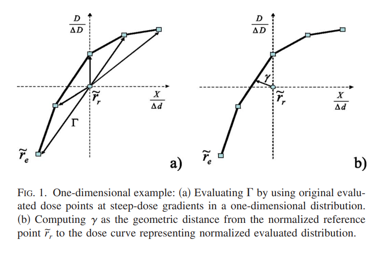
Figure 1a shows the original implementation. Improving on this by increasing interpolation resolution can help with the accuracy of the gamma calculation. However, this improvement is traded for calculation time. The geometric gamma function, shown in Figure 1b, uses a simplex to find the minimum gamma value without interpolation. This results in an improvement in calculation time as well as complexity when the interpolation resolution is medium/high. This also comes at the cost of some more complex math.

Gamma function¶

The gamma function is defined as Equation 4 of the paper:

\[\gamma(r_{e}) = \min_{S \in G_{r}} D(\widetilde{r}_{e}, S)\]

along with equation 6:

\[\overline{D}(p,S) = \min_{\{w_{1},...,w_{k + 1}\}} \left| p - \sum_{i=1}^{k+1} w_{i}v_{i} \right|\]

where \(\{w_{1},...,w_{k + 1}\}\) are the weights of the simplex, \(v_{i}\) are the vertices of the simplex, and \(p\) is the point to evaluate, i.e. \(p = r_{e}\).

The weights are calculated via equation 7:

\[\{w_{1},...,w_{k + 1}\} = (V^{T}V)^{-1}V^{T}P, w_{k+1} = 1 - \sum_{i=1}^{k}w_{i}\]

where \(V\) and \(P\) are calculated via equation 8:

\[\begin{split}V = \begin{Bmatrix} c_{1}(p) - c_{1}(v_{k+1}) \\ \vdots \\ c_{n}(p) - c_{n}(v_{k+1}) \end{Bmatrix}\end{split}\]

\[\begin{split}P = \begin{Bmatrix} c_{1}(v_{1}) - c_{1}(v_{k+1}) & \vdots & c_{1}(v_{k}) - c_{1}(v_{k+1}) \\ \vdots & \ddots & \vdots \\ c_{n}(v_{1}) - c_{n}(v_{k+1}) & \vdots & c_{n}(v_{k}) - c_{n}(v_{k+1}) \end{Bmatrix}\end{split}\]

Also, as stated in the paper, the projection of the point onto the simplex may not be within the bounds of the simplex support. In the 1D case, we can simply take the minimum distance to the closest vertex.

Logic¶

The reference and evaluation distributions are both normalized by the maximum reference value * the dose to agreement parameter.
For each evaluation point \(p\):
1. The vertices of each simplex are found. In the 1D scenario these will always be line segments defined by 2 points. All the points that are within and just beyond the geometric range of the DTA parameter. E.g. if the DTA is 3mm and the evaluation point is at 10mm, the vertices of the reference distribution are found that are within and just beyond 7-13mm. The next-furthest-away reference point away on either side is the first vertex. If the reference distribution was every 0.3mm then the first and last vertices sets would be 6.9-7.2mm, …, 129.9-130.2mm.
2. The distance from \(p\) to each contained simplex is calculated.
3. The minimum distance across simplex evaluations is the gamma value for that point.

Usage¶

Arrays¶

Original Gamma¶

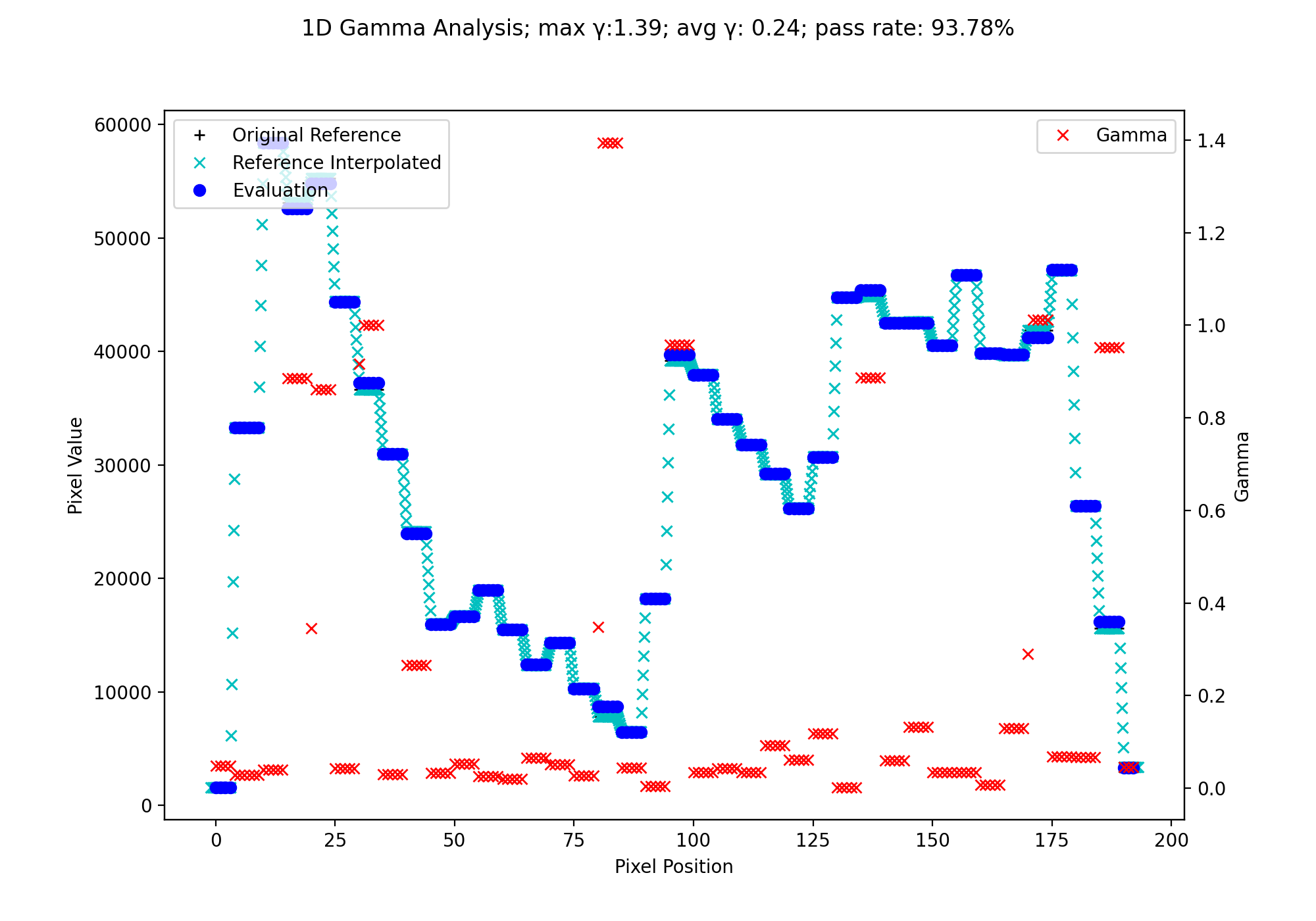
We will use the H&N 1mm, DD example from Agnew & McGarry. Although their data is 2D, we can extract a 1D profile from their data. Below we use the original Low gamma function to calculate gamma for a 1D profile.

import matplotlib.pyplot as plt

from pylinac.core.io import retrieve_demo_file
from pylinac.core.gamma import gamma_1d
from pylinac.core.image import DicomImage

# get the files from the cloud
ref_file = retrieve_demo_file(name='gamma/HN_VMAT_Reference_1mmPx.dcm')
eval_file = retrieve_demo_file(name='gamma/HN_VMAT_Evaluated_1mmPx.dcm')
# load them as DICOM images; we want to use the raw pixels
ref_img = DicomImage(ref_file, raw_pixels=True)
eval_img = DicomImage(eval_file, raw_pixels=True)
# convert the images to float arrays; uints can result in overflow errors
ref_array = ref_img.array.astype(float)
eval_array = eval_img.array.astype(float)
# take a random sample profile through the middle of the images
ref_prof = ref_img[:, 90]
eval_prof = eval_img[:, 90]

# compute the gamma
gamma_map, ref_vals, ref_x_vals = gamma_1d(ref_prof, eval_prof, resolution_factor=7, dose_threshold=0)

# plot the results
fig, ax = plt.subplots(figsize=(10, 7))
ax.plot(ref_prof, 'k+', label='Original Reference', )
ax.plot(ref_x_vals, ref_vals, 'cx', label='Reference Interpolated',)
ax.plot(eval_prof, 'bo', label='Evaluation')
ax.set_ylabel('Pixel Value')
ax.set_xlabel('Pixel Position')
ax.legend(loc='upper left')
g_ax = ax.twinx()
g_ax.plot(gamma_map, 'rx', label='Gamma')
g_ax.legend(loc='upper right')
g_ax.set_ylabel('Gamma')
fig.suptitle(f'1D Gamma Analysis; max \N{Greek Small Letter Gamma}:{gamma_map.max():.2f}; avg \N{Greek Small Letter Gamma}: {gamma_map.mean():.2f}; pass rate: {100*gamma_map[gamma_map <= 1].size/gamma_map.size:.2f}%')
plt.show()

(Source code, png, hires.png, pdf)

Geometric Gamma¶

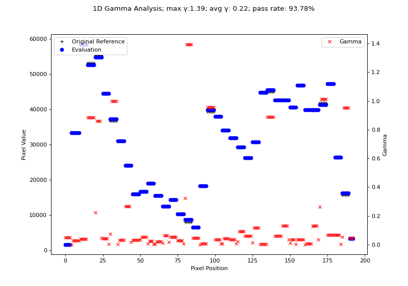
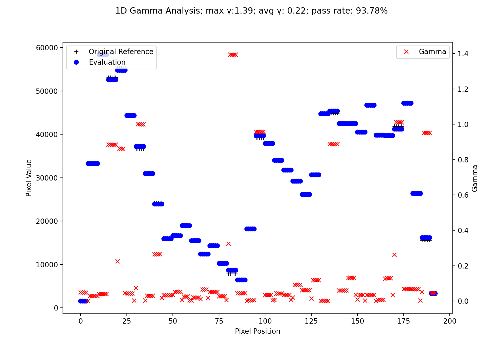
Next, let’s also calculate the geometric gamma for the same data:

import matplotlib.pyplot as plt

from pylinac.core.io import retrieve_demo_file
from pylinac.core.gamma import gamma_geometric
from pylinac.core.image import DicomImage

# get the files from the cloud
ref_file = retrieve_demo_file(name='gamma/HN_VMAT_Reference_1mmPx.dcm')
eval_file = retrieve_demo_file(name='gamma/HN_VMAT_Evaluated_1mmPx.dcm')
# load them as DICOM images; we want to use the raw pixels
ref_img = DicomImage(ref_file, raw_pixels=True)
eval_img = DicomImage(eval_file, raw_pixels=True)
# convert the images to float arrays; uints can result in overflow errors
ref_array = ref_img.array.astype(float)
eval_array = eval_img.array.astype(float)
# take a random sample profile through the middle of the images
ref_prof = ref_img[:, 90]
eval_prof = eval_img[:, 90]

# compute the gamma
gamma_map = gamma_geometric(ref_prof, eval_prof, dose_threshold=0)

# plot the results
fig, ax = plt.subplots(figsize=(10, 7))
ax.plot(ref_prof, 'k+', label='Original Reference')
ax.plot(eval_prof, 'bo', label='Evaluation')
ax.set_ylabel('Pixel Value')
ax.set_xlabel('Pixel Position')
ax.legend(loc='upper left')
g_ax = ax.twinx()
g_ax.plot(gamma_map, 'rx', label='Gamma')
g_ax.legend(loc='upper right')
g_ax.set_ylabel('Gamma')
fig.suptitle(f'1D Gamma Analysis; max \N{Greek Small Letter Gamma}:{gamma_map.max():.2f}; avg \N{Greek Small Letter Gamma}: {gamma_map.mean():.2f}; pass rate: {100*gamma_map[gamma_map <= 1].size/gamma_map.size:.2f}%')
plt.show()

(Source code, png, hires.png, pdf)

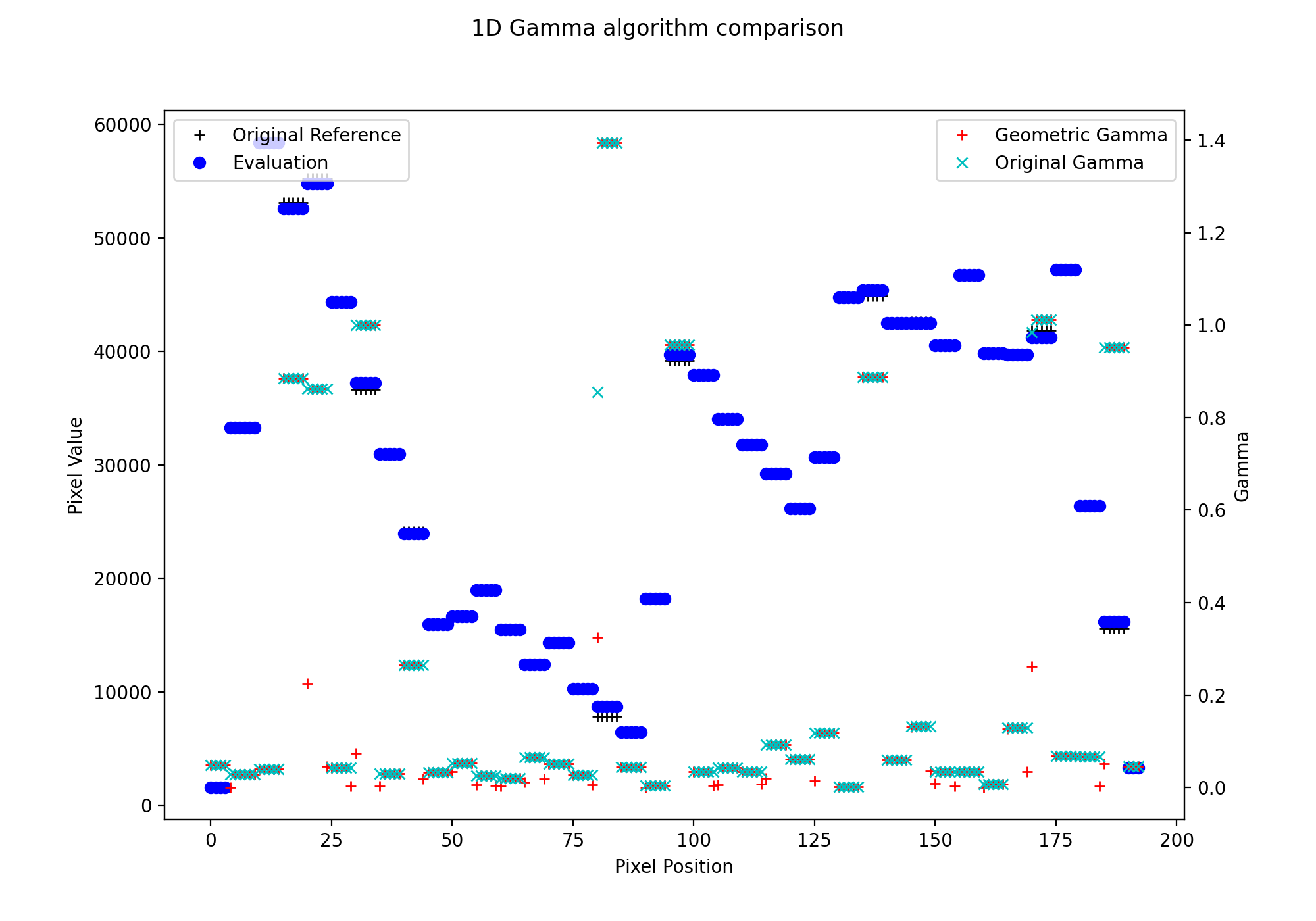
Finally, let’s plot both against each other:

import matplotlib.pyplot as plt

from pylinac.core.io import retrieve_demo_file
from pylinac.core.gamma import gamma_geometric, gamma_1d
from pylinac.core.image import DicomImage

# get the files from the cloud
ref_file = retrieve_demo_file(name='gamma/HN_VMAT_Reference_1mmPx.dcm')
eval_file = retrieve_demo_file(name='gamma/HN_VMAT_Evaluated_1mmPx.dcm')
# load them as DICOM images; we want to use the raw pixels
ref_img = DicomImage(ref_file, raw_pixels=True)
eval_img = DicomImage(eval_file, raw_pixels=True)
# convert the images to float arrays; uints can result in overflow errors
ref_array = ref_img.array.astype(float)
eval_array = eval_img.array.astype(float)
# take a random sample profile through the middle of the images
ref_prof = ref_img[:, 90]
eval_prof = eval_img[:, 90]

# compute the gamma
geometric_gamma_map = gamma_geometric(ref_prof, eval_prof, dose_threshold=0)
gamma_map, _, _ = gamma_1d(ref_prof, eval_prof, resolution_factor=2, dose_threshold=0)

# plot the results
fig, ax = plt.subplots(figsize=(10, 7))
ax.plot(ref_prof, 'k+', label='Original Reference')
ax.plot(eval_prof, 'bo', label='Evaluation')
ax.set_ylabel('Pixel Value')
ax.set_xlabel('Pixel Position')
ax.legend(loc='upper left')
g_ax = ax.twinx()
g_ax.plot(geometric_gamma_map, 'r+', label='Geometric Gamma')
g_ax.plot(gamma_map, 'cx', label='Original Gamma')
g_ax.legend(loc='upper right')
g_ax.set_ylabel('Gamma')
fig.suptitle('1D Gamma algorithm comparison')
plt.show()

(Source code, png, hires.png, pdf)

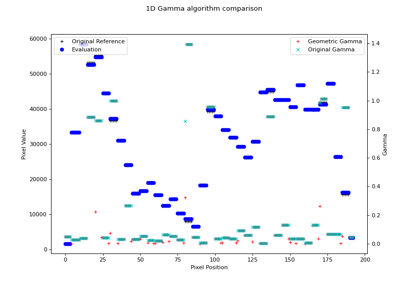
Note that the original gamma is slightly higher than the geometric gamma. This is due to the interpolation. Higher interpolation factors will get closer to the geometric gamma value, but at the cost of calculation time.

Profiles¶

It is also possible to calculate and plot the gamma for a 1D profile via the gamma() method and/or the plot_gamma() method.

Tip

Gamma can only be calculated on “Physical” profiles. If your profile is not physical then the above array-based approach works well.

Warning

Currently, both profiles are geometrically centered before computing the gamma. Know this going in.

Below, let’s generate two profiles from two different synthetic EPIDs (to simulate different resolutions and physical locations) and calculate the gamma between them:

from pylinac.core.profile import FWXMProfilePhysical
from pylinac.core.image_generator import AS1200Image, AS1000Image, GaussianFilterLayer, FilteredFieldLayer

# create the synthetic images
as1000 = AS1000Image()
as1000.add_layer(
    FilteredFieldLayer(field_size_mm=(100, 100))
)
as1000.add_layer(
    GaussianFilterLayer(sigma_mm=2)
)
as1200 = AS1200Image()
as1200.add_layer(
    FilteredFieldLayer(field_size_mm=(100, 100))
)
as1200.add_layer(
    GaussianFilterLayer(sigma_mm=2)
)

# and the profiles
p1200 = as1200.image[640, :]
p1000 = as1000.image[384, :]
p1200_prof = FWXMProfilePhysical(values=p1200, dpmm=1/as1200.pixel_size)
p1000_prof = FWXMProfilePhysical(values=p1000, dpmm=1/as1000.pixel_size)

# compute gamma as a numpy array the same size as the evaluation profile
gamma = p1000_prof.gamma(reference_profile=p1200_prof, dose_to_agreement=1, gamma_cap_value=2)

# we could calculate pass rate, etc from this.
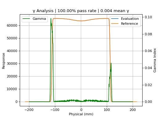
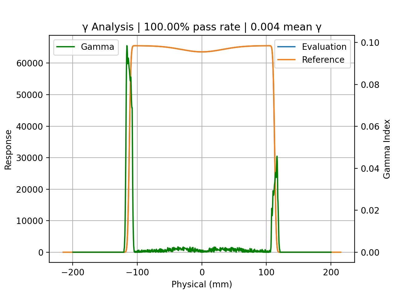
# However, we want to plot it. The helper method does this for us, plotting the profiles and gamma.
p1000_prof.plot_gamma(reference_profile=p1200_prof, dose_to_agreement=1, dose_threshold=0)

(Source code, png, hires.png, pdf)

API¶

pylinac.core.gamma.gamma_geometric(reference: ndarray, evaluation: ndarray, reference_coordinates: ndarray | None = None, evaluation_coordinates: ndarray | None = None, dose_to_agreement: float = 1, distance_to_agreement: float = 1, gamma_cap_value: float = 2, dose_threshold: float = 5, fill_value: float = nan) → ndarray[source]¶

Compute the Ju et al geometric gamma of two 1D profiles/arrays. 2D support will come in the future and should be doable in-place.

Parameters¶

reference: The reference profile.
evaluation: The evaluation profile.
reference_coordinates: The x-values of the reference profile. If None, will be assumed to be evenly spaced from 0 to len(reference).
evaluation_coordinates: The x-values of the evaluation profile. If None, will be assumed to be evenly spaced from 0 to len(evaluation).
dose_to_agreement: The dose to agreement in %. E.g. 1 is 1% of global reference max dose.
distance_to_agreement: The distance to agreement in x-values (generally this should be mm).
gamma_cap_value: The value to cap the gamma at. E.g. a gamma of 5.3 will get capped to 2. Useful for displaying data with a consistent range.
dose_threshold: The dose threshold as a number between 0 and 100 of the % of max dose under which a gamma is not calculated.
fill_value: The value to give pixels that were not calculated because they were under the dose threshold. Default is NaN, but another option would be 0. If NaN, allows the user to calculate mean/median gamma over just the evaluated portion and not be skewed by 0’s that should not be considered.

Returns¶

np.ndarray: The gamma values. The dimensions will be the same as the evaluation profile.

pylinac.core.gamma.gamma_2d(reference: ndarray, evaluation: ndarray, dose_to_agreement: float = 1, distance_to_agreement: int = 1, gamma_cap_value: float = 2, global_dose: bool = True, dose_threshold: float = 5, fill_value: float = nan) → ndarray[source]¶

Compute a 2D gamma of two 2D numpy arrays. This does NOT do size or spatial resolution checking. It performs an element-by-element evaluation. It is the responsibility of the caller to ensure the reference and evaluation have comparable spatial resolution.

The algorithm follows Table I of D. Low’s 2004 paper: Evaluation of the gamma dose distribution comparison method: https://aapm.onlinelibrary.wiley.com/doi/epdf/10.1118/1.1598711

This is similar to the gamma_1d function for profiles, except we must search a 2D grid around the reference point.

Parameters¶

reference: The reference 2D array.
evaluation: The evaluation 2D array.
dose_to_agreement: The dose to agreement in %. E.g. 1 is 1% of global reference max dose.
distance_to_agreement: The distance to agreement in elements. E.g. if the value is 4 this means 4 elements from the reference point under calculation. Must be >0
gamma_cap_value: The value to cap the gamma at. E.g. a gamma of 5.3 will get capped to 2. Useful for displaying data with a consistent range.
global_dose: Whether to evaluate the dose to agreement threshold based on the global max or the dose point under evaluation.
dose_threshold: The dose threshold as a number between 0 and 100 of the % of max dose under which a gamma is not calculated. This is not affected by the global/local dose normalization and the threshold value is evaluated against the global max dose, period.
fill_value: The value to give pixels that were not calculated because they were under the dose threshold. Default is NaN, but another option would be 0. If NaN, allows the user to calculate mean/median gamma over just the evaluated portion and not be skewed by 0’s that should not be considered.

pylinac.core.gamma.gamma_1d(reference: np.ndarray, evaluation: np.ndarray, reference_coordinates: np.ndarray | None = None, evaluation_coordinates: np.ndarray | None = None, dose_to_agreement: float = 1, distance_to_agreement: int = 1, gamma_cap_value: float = 2, global_dose: bool = True, dose_threshold: float = 5, resolution_factor: int = 3, fill_value: float = nan)[source]¶

Perform a 1D gamma of two 1D profiles/arrays.

The algorithm follows Table I of D. Low’s 2004 paper: Evaluation of the gamma dose distribution comparison method: https://aapm.onlinelibrary.wiley.com/doi/epdf/10.1118/1.1598711

Parameters¶

reference: The reference profile.
evaluation: The evaluation profile.
reference_coordinates: The x-values of the reference profile. If None, will be assumed to be evenly spaced from 0 to len(reference).
evaluation_coordinates: The x-values of the evaluation profile. If None, will be assumed to be evenly spaced from 0 to len(evaluation).
dose_to_agreement: The dose to agreement in %. E.g. 1 is 1% of global reference max dose.
distance_to_agreement: The distance to agreement in x-values. If no x-values are passed, this is in elements. If x-values are passed, this is in the units of the x-values. E.g. if the x-values are in mm and the distance to agreement is 1, this is 1 mm. Must be >0.
gamma_cap_value: The value to cap the gamma at. E.g. a gamma of 5.3 will get capped to 2. Useful for displaying data with a consistent range.
global_dose: Whether to evaluate the dose to agreement threshold based on the global max or the dose point under evaluation.
dose_threshold: The dose threshold as a number between 0 and 100 of the % of max dose under which a gamma is not calculated. This is not affected by the global/local dose normalization and the threshold value is evaluated against the global max dose, period.
resolution_factor: The factor by which to resample the reference profile to be compared to the evaluation profile. Depends on the distance to agreement. If the distance to agreement is 1 mm and the resolution factor is 3, the reference profile will be resampled to 0.333 mm resolution. The rule of thumb is to use at least 3x the distance to agreement. Higher factors will increase computation time.
fill_value: The value to give pixels that were not calculated because they were under the dose threshold. Default is NaN, but another option would be 0. If NaN, allows the user to calculate mean/median gamma over just the evaluated portion and not be skewed by 0’s that should not be considered.

Returns¶

np.ndarray: The gamma values. The dimensions will be the same as the evaluation profile.
np.ndarray: The resampled reference profile. Useful for plotting.
np.ndarray: The x-values of the resampled reference profile. Useful for plotting.