CatPhan/CT
Overview
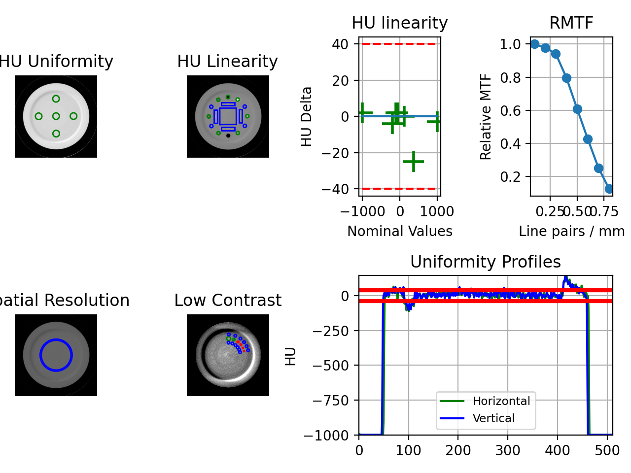
The CatPhan module automatically analyzes DICOM images of a CatPhan 504, 503, or 600 acquired when doing CBCT or CT quality assurance. It can load a folder or zip file that the images are in and automatically correct for translational and rotational errors. It can analyze the HU regions and image scaling (CTP404), the high-contrast line pairs (CTP528) to calculate the modulation transfer function (MTF), the HU uniformity (CTP486), and Low Contrast (CTP515) on the corresponding slices.
Features:
- Automatic phantom registration - Your phantom can be tilted, rotated, or translated–pylinac will automatically register the phantom.
- Automatic testing of all major modules - Major modules are automatically registered and analyzed.
- Any scan protocol - Scan your CatPhan with any protocol; even scan it in a regular CT scanner. Any field size or field extent is allowed.
Running the Demo
To run one of the CatPhan demos, create a script or start an interpreter and input:
from pylinac import CatPhan504
cbct = CatPhan504.run_demo()  # the demo is a Varian high quality head scan
(Source code, png, hires.png, pdf)
Results will be also be printed to the console:
- CatPhan 504 QA Test -
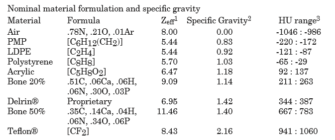
HU Linearity ROIs: Air: -998.0, PMP: -200.0, LDPE: -102.0, Poly: -45.0, Acrylic: 115.0, Delrin: 340.0, Teflon: 997.0
HU Passed?: True
Low contrast visibility: 3.46
Geometric Line Average (mm): 49.95
Geometry Passed?: True
Measured Slice Thickness (mm): 2.499
Slice Thickness Passed? True
Uniformity ROIs: Top: 6.0, Right: -1.0, Bottom: 5.0, Left: 10.0, Center: 14.0
Uniformity index: -1.479
Integral non-uniformity: 0.0075
Uniformity Passed?: True
MTF 50% (lp/mm): 0.56
Low contrast ROIs "seen": 3
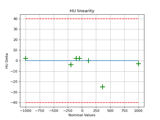
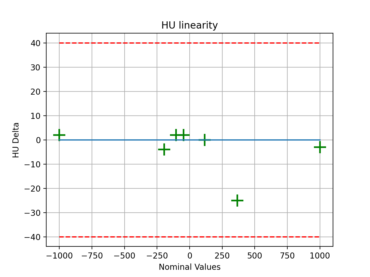
As well, you can plot and save individual pieces of the analysis such as linearity:
(Source code, png, hires.png, pdf)

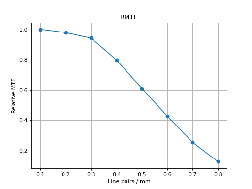
Or the rMTF:
cbct.plot_analyzed_subimage('rmtf')
(Source code, png, hires.png, pdf)

Or generate a PDF report:
cbct.publish_pdf('mycbct.pdf')
Typical Use
CatPhan analysis as done by this module closely follows what is specified in the CatPhan manuals, replacing the need for manual measurements.
There are 4 CatPhan models that pylinac can analyze: CatPhan504, CatPhan503, & CatPhan600, &
CatPhan604, each with their own class in
pylinac. Let’s assume you have the CatPhan504 for this example. Using the other models/classes is exactly
the same except the class name.
from pylinac import CatPhan504 # or import the CatPhan503 or CatPhan600
The minimum needed to get going is to:
Load images – Loading the DICOM images into your CatPhan object is done by passing the images in during construction. The most direct way is to pass in the directory where the images are:
cbct_folder = r"C:/QA Folder/CBCT/June monthly"
mycbct = CatPhan504(cbct_folder)
or load a zip file of the images:
zip_file = r"C:/QA Folder/CBCT/June monthly.zip"
mycbct = CatPhan504.from_zip(zip_file)
You can also use the demo images provided:
mycbct = CatPhan504.from_demo_images()
Analyze the images – Once the folder/images are loaded, tell pylinac to start analyzing the images. See the Algorithm section for details and
analyze`()for analysis options:mycbct.analyze()
View the results – The CatPhan module can print out the summary of results to the console as well as draw a matplotlib image to show where the samples were taken and their values:
# print results to the console
print(mycbct.results())
# view analyzed images
mycbct.plot_analyzed_image()
# save the image
mycbct.save_analyzed_image('mycatphan504.png')
# generate PDF
mycbct.publish_pdf('mycatphan.pdf', open_file=True)  # open the PDF after saving as well.
Advanced Use
Using results_data
Changed in version 3.0.
Using the catphan module in your own scripts? While the analysis results can be printed out,
if you intend on using them elsewhere (e.g. in an API), they can be accessed the easiest by using the results_data() method
which returns a CatphanResult instance.
Note
While the pylinac tooling may change under the hood, this object should remain largely the same and/or expand. Thus, using this is more stable than accessing attrs directly.
Continuing from above:
data = mycbct.results_data()
data.catphan_model
data.ctp404.measured_slice_thickness_mm
# and more

# return as a dict
data_dict = mycbct.results_data(as_dict=True)
data_dict['ctp404']['measured_slice_thickness_mm']
...
Partial scans
While the default behavior of pylinac is to analyze all modules in the scan (in fact it will error out if they aren’t),
the behavior can be customized. Pylinac always has to be aware of the CTP404 module as that’s the reference slice
for everything else. Thus, if the 404 is not in the scan you’re SOL. However, if one of the other modules is not present
you can remove or adjust its offset by subclassing and overloading the modules attr:
from pylinac import CatPhan504  # works for any of the other phantoms too
from pylinac.ct import CTP515, CTP486

class PartialCatPhan504(CatPhan504):
    modules = {
        CTP486: {'offset': -65},
        CTP515: {'offset': -30},
        # the CTP528 was omitted
    }

ct = PartialCatPhan504.from_zip(...)  # use like normal
Examining rMTF
The rMTF can be calculated ad hoc like so. Note that CTP528 must be present (see above):
ct = ... # load a dataset like normal
ct.analyze()
ct.ctp528.mtf.relative_resolution(x=40)  # get the rMTF (lp/mm) at 40% resolution
Customizing module locations
Similar to partial scans, to modify the module location(s), overload the modules attr and edit the offset value.
The value is in mm:
from pylinac import CatPhan504  # works for any of the other phantoms too
from pylinac.ct import CTP515, CTP486, CTP528

# create custom catphan with module locations
class OffsetCatPhan504(CatPhan504):
    modules = {
        CTP486: {'offset': -60},  # normally -65
        CTP528: {'offset': 30},
        CTP515: {'offset': -25},  # normally -30
    }

ct = OffsetCatPhan504.from_zip(...)  # use like normal
Customizing Modules
You can also customize modules themselves in v2.4+. Customization should always be done by subclassing an existing module and overloading the attributes. Then, pass in the new custom module into the parent CatPhan class. The easiest way to get started is copy the relevant attributes from the existing code.
As an example, let’s override the nominal HU values for CTP404.
from pylinac.ct import CatPhan504, CTP404CP504

# first, customize the module
class CustomCTP404(CTP404CP504):
    roi_dist_mm = 58.7  # this is the default value; we repeat here because it's easy to copy from source
    roi_radius_mm = 5  # ditto
    roi_settings = {
        'Air': {'value': -1000, 'angle': -93, 'distance': roi_dist_mm, 'radius': roi_radius_mm},  # changed 'angle' from -90
        'PMP': {'value': -196, 'angle': -120, 'distance': roi_dist_mm, 'radius': roi_radius_mm},
        ...  # add other ROIs as appropriate
    }

# then, pass to the CatPhan model
class CustomCP504(CatPhan504):
    modules = {
        CustomCTP404: {'offset': 0}
        ...  # add other modules here as appropriate
    }

# use like normal
ct = CustomCP504(...)
Warning
If you overload the roi_settings or modules attributes, you are responsible for filling it out completely.
I.e. when you overload it’s not partial. In the above example if you want other CTP modules you must populate them.
Algorithm
The CatPhan module is based on the tests and values given in the respective CatPhan manual. The algorithm works like such:
Allowances
- The images can be any size.
- The phantom can have significant translation in all 3 directions.
- The phantom can have significant roll and moderate yaw and pitch.
Restrictions
Warning
Analysis can fail or give unreliable results if any Restriction is violated.
- All of the modules defined in the
modulesattribute must be within the scan extent.
Pre-Analysis
Determine image properties – Upon load, the image set is analyzed for its DICOM properties to determine mm/pixel spacing, rescale intercept and slope, manufacturer, etc.
Convert to HU – The entire image set is converted from its raw values to HU by applying the rescale intercept and slope which is contained in the DICOM properties.
Find the phantom z-location – Upon loading, all the images are scanned to determine where the HU linearity module (CTP404) is located. This is accomplished by examining each image slice and looking for 2 things:
- If the CatPhan is in the image. At the edges of the scan this may not be true.
- If a circular profile has characteristics like the CTP404 module. If the CatPhan is in the image, a circular profile is taken at the location where the HU linearity regions of interest are located. If the profile contains low, high, and lots of medium values then it is very likely the HU linearity module. All such slices are found and the median slice is set as the HU linearity module location. All other modules are located relative to this position.
Analysis
Determine phantom roll – Precise knowledge of the ROIs to analyze is important, and small changes in rotation could invalidate automatic results. The roll of the phantom is determined by examining the HU module and converting to a binary image. The air holes are then located and the angle of the two holes determines the phantom roll.
Note
For each step below, the “module” analyzed is actually the mean, median, or maximum of 3 slices (+/-1 slice around and including the nominal slice) to ensure robust measurements. Also, for each step/phantom module, the phantom center is determined, which corrects for the phantom pitch and yaw.
Additionally, values tend to be lazy (computed only when asked for), thus the calculations listed may sometimes be performed only when asked for.
Determine HU linearity – The HU module (CTP404) contains several materials with different HU values. Using hardcoded angles (corrected for roll) and radius from the center of the phantom, circular ROIs are sampled which correspond to the HU material regions. The median pixel value of the ROI is the stated HU value. Nominal HU values are taken as the mean of the range given in the manual(s):
Determine HU uniformity – HU uniformity (CTP486) is calculated in a similar manner to HU linearity, but within the CTP486 module/slice.
Calculate Geometry/Scaling – The HU module (CTP404), besides HU materials, also contains several “nodes” which have an accurate spacing (50 mm apart). Again, using hardcoded but corrected angles, the area around the 4 nodes are sampled and then a threshold is applied which identifies the node within the ROI sample. The center of mass of the node is determined and then the space between nodes is calculated.
Calculate Spatial Resolution/MTF – The Spatial Resolution module (CTP528) contains 21 pairs of aluminum bars having varying thickness, which also corresponds to the thickness between the bars. One unique advantage of these bars is that they are all focused on and equally distant to the phantom center. This is taken advantage of by extracting a
CollapsedCircleProfileabout the line pairs. The peaks and valleys of the profile are located; peaks and valleys of each line pair are used to calculated the MTF. The relative MTF (i.e. normalized to the first line pair) is then calculated from these values.Calculate Low Contrast Resolution – Low contrast is inherently difficult to determine since detectability of humans is not simply contrast based. Pylinac’s analysis uses both the contrast value of the ROI as well as the ROI size to compute a “detectability” score. ROIs above the score are said to be “seen”, while those below are not seen. Only the 1.0% supra-slice ROIs are examined. Two background ROIs are sampled on either side of the ROI contrast set. See Visibility for equation details.
Calculate Slice Thickness – Slice thickness is measured by determining the FWHM of the wire ramps in the CTP404 module. A profile of the area around each wire ramp is taken, and the FWHM is determined from the profile. Based on testing, the FWHM is not always perfectly detected and may not “catch” the profile, giving an undervalued representation. Thus, the two longest profiles are averaged and the value is converted from pixels to mm and multiplied by 0.42.
Post-Analysis
- Test if values are within tolerance – For each module, the determined values are compared with the nominal values. If the difference between the two is below the specified tolerance then the module passes.
Troubleshooting
First, check the general Troubleshooting section. Most problems in this module revolve around getting the data loaded.
- If you’re having trouble getting your dataset in, make sure you’re loading the whole dataset. Also make sure you’ve scanned the whole phantom.
- Make sure there are no external markers on the CatPhan (e.g. BBs), otherwise the localization algorithm will not be able to properly locate the phantom within the image.
- Ensure that the FOV is large enough to encompass the entire phantom. If the scan is cutting off the phantom in any way it will not identify it.
- The phantom should never touch the edge of an image, see above point.
- Make sure you’re loading the right CatPhan class. I.e. using a CatPhan600 class on a CatPhan504 scan may result in errors or erroneous results.
API Documentation
Main classes
These are the classes a typical user may interface with.
-
class
pylinac.ct.CatPhan504(folderpath: Union[str, Sequence[T_co]], check_uid: bool = True)[source]¶ Bases:
pylinac.ct.CatPhanBaseA class for loading and analyzing CT DICOM files of a CatPhan 504. Can be from a CBCT or CT scanner Analyzes: Uniformity (CTP486), High-Contrast Spatial Resolution (CTP528), Image Scaling & HU Linearity (CTP404), and Low contrast (CTP515).
Parameters: - folderpath (str or list of strings) – String that points to the CBCT image folder location.
- check_uid (bool) – Whether to enforce raising an error if more than one UID is found in the dataset.
Raises: NotADirectoryError– If folder str passed is not a valid directory.FileNotFoundError– If no CT images are found in the folder
-
static
run_demo(show: bool = True)[source]¶ Run the CBCT demo using high-quality head protocol images.
-
analyze(hu_tolerance: Union[int, float] = 40, scaling_tolerance: Union[int, float] = 1, thickness_tolerance: Union[int, float] = 0.2, low_contrast_tolerance: Union[int, float] = 1, cnr_threshold: Union[int, float] = 15, zip_after: bool = False, contrast_method: Union[pylinac.core.roi.Contrast, str] = <Contrast.MICHELSON: 'Michelson'>, visibility_threshold: float = 0.15)¶ Single-method full analysis of CBCT DICOM files.
Parameters: - hu_tolerance (int) – The HU tolerance value for both HU uniformity and linearity.
- scaling_tolerance (float, int) – The scaling tolerance in mm of the geometric nodes on the HU linearity slice (CTP404 module).
- thickness_tolerance (float, int) –
The tolerance of the thickness calculation in mm, based on the wire ramps in the CTP404 module.
Warning
Thickness accuracy degrades with image noise; i.e. low mAs images are less accurate.
- low_contrast_tolerance (int) – The number of low-contrast bubbles needed to be “seen” to pass.
- cnr_threshold (float, int) –
Deprecated since version 3.0: Use visibility parameter instead.
The threshold for “detecting” low-contrast image. See RTD for calculation info.
- zip_after (bool) – If the CT images were not compressed before analysis and this is set to true, pylinac will compress the analyzed images into a ZIP archive.
- contrast_method – The contrast equation to use. See Low contrast.
- visibility_threshold – The threshold for detecting low-contrast ROIs. Use instead of
cnr_threshold. Follows the Rose equation. See Visibility.
-
catphan_size¶ The expected size of the phantom in pixels, based on a 20cm wide phantom.
-
find_origin_slice() → int¶ Using a brute force search of the images, find the median HU linearity slice.
This method walks through all the images and takes a collapsed circle profile where the HU linearity ROIs are. If the profile contains both low (<800) and high (>800) HU values and most values are the same (i.e. it’s not an artifact), then it can be assumed it is an HU linearity slice. The median of all applicable slices is the center of the HU slice.
Returns: The middle slice of the HU linearity module. Return type: int
-
find_phantom_roll() → float¶ Determine the “roll” of the phantom.
This algorithm uses the two air bubbles in the HU slice and the resulting angle between them.
Returns: float Return type: the angle of the phantom in degrees.
-
classmethod
from_demo_images()¶ Construct a CBCT object from the demo images.
-
classmethod
from_url(url: str, check_uid: bool = True)¶ Instantiate a CBCT object from a URL pointing to a .zip object.
Parameters: - url (str) – URL pointing to a zip archive of CBCT images.
- check_uid (bool) – Whether to enforce raising an error if more than one UID is found in the dataset.
-
classmethod
from_zip(zip_file: Union[str, zipfile.ZipFile, BinaryIO], check_uid: bool = True)¶ Construct a CBCT object and pass the zip file.
Parameters: - zip_file (str, ZipFile) – Path to the zip file or a ZipFile object.
- check_uid (bool) – Whether to enforce raising an error if more than one UID is found in the dataset.
Raises: - FileExistsError : If zip_file passed was not a legitimate zip file.
- FileNotFoundError : If no CT images are found in the folder
-
localize() → None¶ Find the slice number of the catphan’s HU linearity module and roll angle
-
mm_per_pixel¶ The millimeters per pixel of the DICOM images.
-
num_images¶ The number of images loaded.
-
plot_analyzed_image(show: bool = True) → None¶ Plot the images used in the calculate and summary data.
Parameters: show (bool) – Whether to plot the image or not.
-
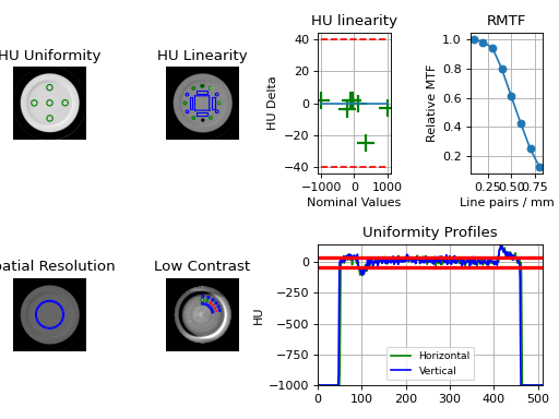
plot_analyzed_subimage(subimage: str = 'hu', delta: bool = True, show: bool = True) → None¶ Plot a specific component of the CBCT analysis.
Parameters: - subimage ({'hu', 'un', 'sp', 'lc', 'mtf', 'lin', 'prof'}) –
The subcomponent to plot. Values must contain one of the following letter combinations. E.g.
linearity,linear, andlinwill all draw the HU linearity values.hudraws the HU linearity image.undraws the HU uniformity image.spdraws the Spatial Resolution image.mtfdraws the RMTF plot.lindraws the HU linearity values. Used withdelta.profdraws the HU uniformity profiles.
- delta (bool) – Only for use with
lin. Whether to plot the HU delta or actual values. - show (bool) – Whether to actually show the plot.
- subimage ({'hu', 'un', 'sp', 'lc', 'mtf', 'lin', 'prof'}) –
-
publish_pdf(filename: str, notes: str = None, open_file: bool = False, metadata: Optional[dict] = None) → None¶ Publish (print) a PDF containing the analysis and quantitative results.
Parameters: - filename ((str, file-like object}) – The file to write the results to.
- notes (str, list of strings) – Text; if str, prints single line. If list of strings, each list item is printed on its own line.
- open_file (bool) – Whether to open the file using the default program after creation.
- metadata (dict) – Extra data to be passed and shown in the PDF. The key and value will be shown with a colon. E.g. passing {‘Author’: ‘James’, ‘Unit’: ‘TrueBeam’} would result in text in the PDF like: ————– Author: James Unit: TrueBeam ————–
-
results() → str¶ Return the results of the analysis as a string. Use with print().
-
results_data(as_dict=False) → Union[pylinac.ct.CatphanResult, dict]¶ Present the results data and metadata as a dataclass or dict. The default return type is a dataclass.
-
save_analyzed_image(filename: str, **kwargs) → None¶ Save the analyzed summary plot.
Parameters: - filename (str, file object) – The name of the file to save the image to.
- kwargs – Any valid matplotlib kwargs.
-
save_analyzed_subimage(filename: Union[str, BinaryIO], subimage: str = 'hu', **kwargs)¶ Save a component image to file.
Parameters: - filename (str, file object) – The file to write the image to.
- subimage (str) – See
plot_analyzed_subimage()for parameter info.
-
class
pylinac.ct.CatPhan503(folderpath: Union[str, Sequence[T_co]], check_uid: bool = True)[source]¶ Bases:
pylinac.ct.CatPhanBaseA class for loading and analyzing CT DICOM files of a CatPhan 503. Analyzes: Uniformity (CTP486), High-Contrast Spatial Resolution (CTP528), Image Scaling & HU Linearity (CTP404).
Parameters: - folderpath (str or list of strings) – String that points to the CBCT image folder location.
- check_uid (bool) – Whether to enforce raising an error if more than one UID is found in the dataset.
Raises: NotADirectoryError– If folder str passed is not a valid directory.FileNotFoundError– If no CT images are found in the folder
-
static
run_demo(show: bool = True)[source]¶ Run the CBCT demo using high-quality head protocol images.
-
analyze(hu_tolerance: Union[int, float] = 40, scaling_tolerance: Union[int, float] = 1, thickness_tolerance: Union[int, float] = 0.2, low_contrast_tolerance: Union[int, float] = 1, cnr_threshold: Union[int, float] = 15, zip_after: bool = False, contrast_method: Union[pylinac.core.roi.Contrast, str] = <Contrast.MICHELSON: 'Michelson'>, visibility_threshold: float = 0.15)¶ Single-method full analysis of CBCT DICOM files.
Parameters: - hu_tolerance (int) – The HU tolerance value for both HU uniformity and linearity.
- scaling_tolerance (float, int) – The scaling tolerance in mm of the geometric nodes on the HU linearity slice (CTP404 module).
- thickness_tolerance (float, int) –
The tolerance of the thickness calculation in mm, based on the wire ramps in the CTP404 module.
Warning
Thickness accuracy degrades with image noise; i.e. low mAs images are less accurate.
- low_contrast_tolerance (int) – The number of low-contrast bubbles needed to be “seen” to pass.
- cnr_threshold (float, int) –
Deprecated since version 3.0: Use visibility parameter instead.
The threshold for “detecting” low-contrast image. See RTD for calculation info.
- zip_after (bool) – If the CT images were not compressed before analysis and this is set to true, pylinac will compress the analyzed images into a ZIP archive.
- contrast_method – The contrast equation to use. See Low contrast.
- visibility_threshold – The threshold for detecting low-contrast ROIs. Use instead of
cnr_threshold. Follows the Rose equation. See Visibility.
-
catphan_size¶ The expected size of the phantom in pixels, based on a 20cm wide phantom.
-
find_origin_slice() → int¶ Using a brute force search of the images, find the median HU linearity slice.
This method walks through all the images and takes a collapsed circle profile where the HU linearity ROIs are. If the profile contains both low (<800) and high (>800) HU values and most values are the same (i.e. it’s not an artifact), then it can be assumed it is an HU linearity slice. The median of all applicable slices is the center of the HU slice.
Returns: The middle slice of the HU linearity module. Return type: int
-
find_phantom_roll() → float¶ Determine the “roll” of the phantom.
This algorithm uses the two air bubbles in the HU slice and the resulting angle between them.
Returns: float Return type: the angle of the phantom in degrees.
-
classmethod
from_demo_images()¶ Construct a CBCT object from the demo images.
-
classmethod
from_url(url: str, check_uid: bool = True)¶ Instantiate a CBCT object from a URL pointing to a .zip object.
Parameters: - url (str) – URL pointing to a zip archive of CBCT images.
- check_uid (bool) – Whether to enforce raising an error if more than one UID is found in the dataset.
-
classmethod
from_zip(zip_file: Union[str, zipfile.ZipFile, BinaryIO], check_uid: bool = True)¶ Construct a CBCT object and pass the zip file.
Parameters: - zip_file (str, ZipFile) – Path to the zip file or a ZipFile object.
- check_uid (bool) – Whether to enforce raising an error if more than one UID is found in the dataset.
Raises: - FileExistsError : If zip_file passed was not a legitimate zip file.
- FileNotFoundError : If no CT images are found in the folder
-
localize() → None¶ Find the slice number of the catphan’s HU linearity module and roll angle
-
mm_per_pixel¶ The millimeters per pixel of the DICOM images.
-
num_images¶ The number of images loaded.
-
plot_analyzed_image(show: bool = True) → None¶ Plot the images used in the calculate and summary data.
Parameters: show (bool) – Whether to plot the image or not.
-
plot_analyzed_subimage(subimage: str = 'hu', delta: bool = True, show: bool = True) → None¶ Plot a specific component of the CBCT analysis.
Parameters: - subimage ({'hu', 'un', 'sp', 'lc', 'mtf', 'lin', 'prof'}) –
The subcomponent to plot. Values must contain one of the following letter combinations. E.g.
linearity,linear, andlinwill all draw the HU linearity values.hudraws the HU linearity image.undraws the HU uniformity image.spdraws the Spatial Resolution image.mtfdraws the RMTF plot.lindraws the HU linearity values. Used withdelta.profdraws the HU uniformity profiles.
- delta (bool) – Only for use with
lin. Whether to plot the HU delta or actual values. - show (bool) – Whether to actually show the plot.
- subimage ({'hu', 'un', 'sp', 'lc', 'mtf', 'lin', 'prof'}) –
-
publish_pdf(filename: str, notes: str = None, open_file: bool = False, metadata: Optional[dict] = None) → None¶ Publish (print) a PDF containing the analysis and quantitative results.
Parameters: - filename ((str, file-like object}) – The file to write the results to.
- notes (str, list of strings) – Text; if str, prints single line. If list of strings, each list item is printed on its own line.
- open_file (bool) – Whether to open the file using the default program after creation.
- metadata (dict) – Extra data to be passed and shown in the PDF. The key and value will be shown with a colon. E.g. passing {‘Author’: ‘James’, ‘Unit’: ‘TrueBeam’} would result in text in the PDF like: ————– Author: James Unit: TrueBeam ————–
-
results() → str¶ Return the results of the analysis as a string. Use with print().
-
results_data(as_dict=False) → Union[pylinac.ct.CatphanResult, dict]¶ Present the results data and metadata as a dataclass or dict. The default return type is a dataclass.
-
save_analyzed_image(filename: str, **kwargs) → None¶ Save the analyzed summary plot.
Parameters: - filename (str, file object) – The name of the file to save the image to.
- kwargs – Any valid matplotlib kwargs.
-
save_analyzed_subimage(filename: Union[str, BinaryIO], subimage: str = 'hu', **kwargs)¶ Save a component image to file.
Parameters: - filename (str, file object) – The file to write the image to.
- subimage (str) – See
plot_analyzed_subimage()for parameter info.
-
class
pylinac.ct.CatPhan600(folderpath: Union[str, Sequence[T_co]], check_uid: bool = True)[source]¶ Bases:
pylinac.ct.CatPhanBaseA class for loading and analyzing CT DICOM files of a CatPhan 600. Analyzes: Uniformity (CTP486), High-Contrast Spatial Resolution (CTP528), Image Scaling & HU Linearity (CTP404), and Low contrast (CTP515).
Parameters: - folderpath (str or list of strings) – String that points to the CBCT image folder location.
- check_uid (bool) – Whether to enforce raising an error if more than one UID is found in the dataset.
Raises: NotADirectoryError– If folder str passed is not a valid directory.FileNotFoundError– If no CT images are found in the folder
-
analyze(hu_tolerance: Union[int, float] = 40, scaling_tolerance: Union[int, float] = 1, thickness_tolerance: Union[int, float] = 0.2, low_contrast_tolerance: Union[int, float] = 1, cnr_threshold: Union[int, float] = 15, zip_after: bool = False, contrast_method: Union[pylinac.core.roi.Contrast, str] = <Contrast.MICHELSON: 'Michelson'>, visibility_threshold: float = 0.15)¶ Single-method full analysis of CBCT DICOM files.
Parameters: - hu_tolerance (int) – The HU tolerance value for both HU uniformity and linearity.
- scaling_tolerance (float, int) – The scaling tolerance in mm of the geometric nodes on the HU linearity slice (CTP404 module).
- thickness_tolerance (float, int) –
The tolerance of the thickness calculation in mm, based on the wire ramps in the CTP404 module.
Warning
Thickness accuracy degrades with image noise; i.e. low mAs images are less accurate.
- low_contrast_tolerance (int) – The number of low-contrast bubbles needed to be “seen” to pass.
- cnr_threshold (float, int) –
Deprecated since version 3.0: Use visibility parameter instead.
The threshold for “detecting” low-contrast image. See RTD for calculation info.
- zip_after (bool) – If the CT images were not compressed before analysis and this is set to true, pylinac will compress the analyzed images into a ZIP archive.
- contrast_method – The contrast equation to use. See Low contrast.
- visibility_threshold – The threshold for detecting low-contrast ROIs. Use instead of
cnr_threshold. Follows the Rose equation. See Visibility.
-
catphan_size¶ The expected size of the phantom in pixels, based on a 20cm wide phantom.
-
find_origin_slice() → int¶ Using a brute force search of the images, find the median HU linearity slice.
This method walks through all the images and takes a collapsed circle profile where the HU linearity ROIs are. If the profile contains both low (<800) and high (>800) HU values and most values are the same (i.e. it’s not an artifact), then it can be assumed it is an HU linearity slice. The median of all applicable slices is the center of the HU slice.
Returns: The middle slice of the HU linearity module. Return type: int
-
find_phantom_roll() → float¶ Determine the “roll” of the phantom.
This algorithm uses the two air bubbles in the HU slice and the resulting angle between them.
Returns: float Return type: the angle of the phantom in degrees.
-
classmethod
from_demo_images()¶ Construct a CBCT object from the demo images.
-
classmethod
from_url(url: str, check_uid: bool = True)¶ Instantiate a CBCT object from a URL pointing to a .zip object.
Parameters: - url (str) – URL pointing to a zip archive of CBCT images.
- check_uid (bool) – Whether to enforce raising an error if more than one UID is found in the dataset.
-
classmethod
from_zip(zip_file: Union[str, zipfile.ZipFile, BinaryIO], check_uid: bool = True)¶ Construct a CBCT object and pass the zip file.
Parameters: - zip_file (str, ZipFile) – Path to the zip file or a ZipFile object.
- check_uid (bool) – Whether to enforce raising an error if more than one UID is found in the dataset.
Raises: - FileExistsError : If zip_file passed was not a legitimate zip file.
- FileNotFoundError : If no CT images are found in the folder
-
localize() → None¶ Find the slice number of the catphan’s HU linearity module and roll angle
-
mm_per_pixel¶ The millimeters per pixel of the DICOM images.
-
num_images¶ The number of images loaded.
-
plot_analyzed_image(show: bool = True) → None¶ Plot the images used in the calculate and summary data.
Parameters: show (bool) – Whether to plot the image or not.
-
plot_analyzed_subimage(subimage: str = 'hu', delta: bool = True, show: bool = True) → None¶ Plot a specific component of the CBCT analysis.
Parameters: - subimage ({'hu', 'un', 'sp', 'lc', 'mtf', 'lin', 'prof'}) –
The subcomponent to plot. Values must contain one of the following letter combinations. E.g.
linearity,linear, andlinwill all draw the HU linearity values.hudraws the HU linearity image.undraws the HU uniformity image.spdraws the Spatial Resolution image.mtfdraws the RMTF plot.lindraws the HU linearity values. Used withdelta.profdraws the HU uniformity profiles.
- delta (bool) – Only for use with
lin. Whether to plot the HU delta or actual values. - show (bool) – Whether to actually show the plot.
- subimage ({'hu', 'un', 'sp', 'lc', 'mtf', 'lin', 'prof'}) –
-
publish_pdf(filename: str, notes: str = None, open_file: bool = False, metadata: Optional[dict] = None) → None¶ Publish (print) a PDF containing the analysis and quantitative results.
Parameters: - filename ((str, file-like object}) – The file to write the results to.
- notes (str, list of strings) – Text; if str, prints single line. If list of strings, each list item is printed on its own line.
- open_file (bool) – Whether to open the file using the default program after creation.
- metadata (dict) – Extra data to be passed and shown in the PDF. The key and value will be shown with a colon. E.g. passing {‘Author’: ‘James’, ‘Unit’: ‘TrueBeam’} would result in text in the PDF like: ————– Author: James Unit: TrueBeam ————–
-
results() → str¶ Return the results of the analysis as a string. Use with print().
-
results_data(as_dict=False) → Union[pylinac.ct.CatphanResult, dict]¶ Present the results data and metadata as a dataclass or dict. The default return type is a dataclass.
-
save_analyzed_image(filename: str, **kwargs) → None¶ Save the analyzed summary plot.
Parameters: - filename (str, file object) – The name of the file to save the image to.
- kwargs – Any valid matplotlib kwargs.
-
save_analyzed_subimage(filename: Union[str, BinaryIO], subimage: str = 'hu', **kwargs)¶ Save a component image to file.
Parameters: - filename (str, file object) – The file to write the image to.
- subimage (str) – See
plot_analyzed_subimage()for parameter info.
-
class
pylinac.ct.CatPhan604(folderpath: Union[str, Sequence[T_co]], check_uid: bool = True)[source]¶ Bases:
pylinac.ct.CatPhanBaseA class for loading and analyzing CT DICOM files of a CatPhan 604. Can be from a CBCT or CT scanner Analyzes: Uniformity (CTP486), High-Contrast Spatial Resolution (CTP528), Image Scaling & HU Linearity (CTP404), and Low contrast (CTP515).
Parameters: - folderpath (str or list of strings) – String that points to the CBCT image folder location.
- check_uid (bool) – Whether to enforce raising an error if more than one UID is found in the dataset.
Raises: NotADirectoryError– If folder str passed is not a valid directory.FileNotFoundError– If no CT images are found in the folder
-
static
run_demo(show: bool = True)[source]¶ Run the CBCT demo using high-quality head protocol images.
-
analyze(hu_tolerance: Union[int, float] = 40, scaling_tolerance: Union[int, float] = 1, thickness_tolerance: Union[int, float] = 0.2, low_contrast_tolerance: Union[int, float] = 1, cnr_threshold: Union[int, float] = 15, zip_after: bool = False, contrast_method: Union[pylinac.core.roi.Contrast, str] = <Contrast.MICHELSON: 'Michelson'>, visibility_threshold: float = 0.15)¶ Single-method full analysis of CBCT DICOM files.
Parameters: - hu_tolerance (int) – The HU tolerance value for both HU uniformity and linearity.
- scaling_tolerance (float, int) – The scaling tolerance in mm of the geometric nodes on the HU linearity slice (CTP404 module).
- thickness_tolerance (float, int) –
The tolerance of the thickness calculation in mm, based on the wire ramps in the CTP404 module.
Warning
Thickness accuracy degrades with image noise; i.e. low mAs images are less accurate.
- low_contrast_tolerance (int) – The number of low-contrast bubbles needed to be “seen” to pass.
- cnr_threshold (float, int) –
Deprecated since version 3.0: Use visibility parameter instead.
The threshold for “detecting” low-contrast image. See RTD for calculation info.
- zip_after (bool) – If the CT images were not compressed before analysis and this is set to true, pylinac will compress the analyzed images into a ZIP archive.
- contrast_method – The contrast equation to use. See Low contrast.
- visibility_threshold – The threshold for detecting low-contrast ROIs. Use instead of
cnr_threshold. Follows the Rose equation. See Visibility.
-
catphan_size¶ The expected size of the phantom in pixels, based on a 20cm wide phantom.
-
find_origin_slice() → int¶ Using a brute force search of the images, find the median HU linearity slice.
This method walks through all the images and takes a collapsed circle profile where the HU linearity ROIs are. If the profile contains both low (<800) and high (>800) HU values and most values are the same (i.e. it’s not an artifact), then it can be assumed it is an HU linearity slice. The median of all applicable slices is the center of the HU slice.
Returns: The middle slice of the HU linearity module. Return type: int
-
find_phantom_roll() → float¶ Determine the “roll” of the phantom.
This algorithm uses the two air bubbles in the HU slice and the resulting angle between them.
Returns: float Return type: the angle of the phantom in degrees.
-
classmethod
from_demo_images()¶ Construct a CBCT object from the demo images.
-
classmethod
from_url(url: str, check_uid: bool = True)¶ Instantiate a CBCT object from a URL pointing to a .zip object.
Parameters: - url (str) – URL pointing to a zip archive of CBCT images.
- check_uid (bool) – Whether to enforce raising an error if more than one UID is found in the dataset.
-
classmethod
from_zip(zip_file: Union[str, zipfile.ZipFile, BinaryIO], check_uid: bool = True)¶ Construct a CBCT object and pass the zip file.
Parameters: - zip_file (str, ZipFile) – Path to the zip file or a ZipFile object.
- check_uid (bool) – Whether to enforce raising an error if more than one UID is found in the dataset.
Raises: - FileExistsError : If zip_file passed was not a legitimate zip file.
- FileNotFoundError : If no CT images are found in the folder
-
localize() → None¶ Find the slice number of the catphan’s HU linearity module and roll angle
-
mm_per_pixel¶ The millimeters per pixel of the DICOM images.
-
num_images¶ The number of images loaded.
-
plot_analyzed_image(show: bool = True) → None¶ Plot the images used in the calculate and summary data.
Parameters: show (bool) – Whether to plot the image or not.
-
plot_analyzed_subimage(subimage: str = 'hu', delta: bool = True, show: bool = True) → None¶ Plot a specific component of the CBCT analysis.
Parameters: - subimage ({'hu', 'un', 'sp', 'lc', 'mtf', 'lin', 'prof'}) –
The subcomponent to plot. Values must contain one of the following letter combinations. E.g.
linearity,linear, andlinwill all draw the HU linearity values.hudraws the HU linearity image.undraws the HU uniformity image.spdraws the Spatial Resolution image.mtfdraws the RMTF plot.lindraws the HU linearity values. Used withdelta.profdraws the HU uniformity profiles.
- delta (bool) – Only for use with
lin. Whether to plot the HU delta or actual values. - show (bool) – Whether to actually show the plot.
- subimage ({'hu', 'un', 'sp', 'lc', 'mtf', 'lin', 'prof'}) –
-
publish_pdf(filename: str, notes: str = None, open_file: bool = False, metadata: Optional[dict] = None) → None¶ Publish (print) a PDF containing the analysis and quantitative results.
Parameters: - filename ((str, file-like object}) – The file to write the results to.
- notes (str, list of strings) – Text; if str, prints single line. If list of strings, each list item is printed on its own line.
- open_file (bool) – Whether to open the file using the default program after creation.
- metadata (dict) – Extra data to be passed and shown in the PDF. The key and value will be shown with a colon. E.g. passing {‘Author’: ‘James’, ‘Unit’: ‘TrueBeam’} would result in text in the PDF like: ————– Author: James Unit: TrueBeam ————–
-
results() → str¶ Return the results of the analysis as a string. Use with print().
-
results_data(as_dict=False) → Union[pylinac.ct.CatphanResult, dict]¶ Present the results data and metadata as a dataclass or dict. The default return type is a dataclass.
-
save_analyzed_image(filename: str, **kwargs) → None¶ Save the analyzed summary plot.
Parameters: - filename (str, file object) – The name of the file to save the image to.
- kwargs – Any valid matplotlib kwargs.
-
save_analyzed_subimage(filename: Union[str, BinaryIO], subimage: str = 'hu', **kwargs)¶ Save a component image to file.
Parameters: - filename (str, file object) – The file to write the image to.
- subimage (str) – See
plot_analyzed_subimage()for parameter info.
-
class
pylinac.ct.CatphanResult(catphan_model: str, catphan_roll_deg: float, origin_slice: int, num_images: int, ctp404: pylinac.ct.CTP404Result, ctp486: Optional[pylinac.ct.CTP486Result] = None, ctp528: Optional[pylinac.ct.CTP528Result] = None, ctp515: Optional[pylinac.ct.CTP515Result] = None)[source]¶ Bases:
pylinac.core.utilities.ResultBaseThis class should not be called directly. It is returned by the
results_data()method. It is a dataclass under the hood and thus comes with all the dunder magic.Use the following attributes as normal class attributes.
-
catphan_model= None
-
catphan_roll_deg= None
-
origin_slice= None
-
num_images= None
-
ctp404= None
-
ctp486= None
-
ctp528= None
-
ctp515= None
-
-
class
pylinac.ct.CTP404Result(offset: int, low_contrast_visibility: float, thickness_passed: bool, measured_slice_thickness_mm: float, thickness_num_slices_combined: int, geometry_passed: bool, avg_line_distance_mm: float, line_distances_mm: List[float], hu_linearity_passed: bool, hu_tolerance: float, hu_rois: Dict[str, pylinac.ct.ROIResult])[source]¶ Bases:
objectThis class should not be called directly. It is returned by the
results_data()method. It is a dataclass under the hood and thus comes with all the dunder magic.Use the following attributes as normal class attributes.
-
offset= None
-
low_contrast_visibility= None
-
thickness_passed= None
-
measured_slice_thickness_mm= None
-
thickness_num_slices_combined= None
-
geometry_passed= None
-
avg_line_distance_mm= None
-
line_distances_mm= None
-
hu_linearity_passed= None
-
hu_tolerance= None
-
hu_rois= None
-
-
class
pylinac.ct.CTP528Result(start_angle_radians: float, mtf_lp_mm: dict, roi_settings: dict)[source]¶ Bases:
objectThis class should not be called directly. It is returned by the
results_data()method. It is a dataclass under the hood and thus comes with all the dunder magic.Use the following attributes as normal class attributes.
-
start_angle_radians= None
-
mtf_lp_mm= None
-
roi_settings= None
-
-
class
pylinac.ct.CTP515Result(cnr_threshold: float, num_rois_seen: int, roi_settings: dict)[source]¶ Bases:
objectThis class should not be called directly. It is returned by the
results_data()method. It is a dataclass under the hood and thus comes with all the dunder magic.Use the following attributes as normal class attributes.
-
cnr_threshold= None
-
num_rois_seen= None
-
roi_settings= None
-
-
class
pylinac.ct.CTP486Result(uniformity_index: float, integral_non_uniformity: float, passed: bool)[source]¶ Bases:
objectThis class should not be called directly. It is returned by the
results_data()method. It is a dataclass under the hood and thus comes with all the dunder magic.Use the following attributes as normal class attributes.
-
uniformity_index= None
-
integral_non_uniformity= None
-
passed= None
-
-
class
pylinac.ct.ROIResult(name: str, value: float, difference: float, nominal_value: float, passed: bool)[source]¶ Bases:
objectThis class should not be called directly. It is returned by the
results_data()method. It is a dataclass under the hood and thus comes with all the dunder magic.Use the following attributes as normal class attributes.
-
name= None
-
value= None
-
difference= None
-
nominal_value= None
-
passed= None
-
Module classes (CTP404, etc)
-
class
pylinac.ct.Slice(catphan, slice_num: Optional[int] = None, combine: bool = True, combine_method: str = 'mean', num_slices: int = 0)[source]¶ Bases:
objectBase class for analyzing specific slices of a CBCT dicom set.
Parameters: - catphan (~pylinac.cbct.CatPhanBase instance.) –
- slice_num (int) – The slice number of the DICOM array desired. If None, will use the
slice_numproperty of subclass. - combine (bool) – If True, combines the slices +/-
num_slicesaround the slice of interest to improve signal/noise. - combine_method ({'mean', 'max'}) – How to combine the slices if
combineis True. - num_slices (int) – The number of slices on either side of the nominal slice to combine to improve signal/noise; only
applicable if
combineis True.
-
phan_center¶ Determine the location of the center of the phantom.
The image is analyzed to see if: 1) the CatPhan is even in the image (if there were any ROIs detected) 2) an ROI is within the size criteria of the catphan 3) the ROI area that is filled compared to the bounding box area is close to that of a circle
Raises: ValueError– If any of the above conditions are not met.
-
class
pylinac.ct.CatPhanModule(catphan, tolerance: Optional[float], offset: int = 0)[source]¶ Bases:
pylinac.ct.SliceBase class for a CTP module.
-
roi_dist_mm¶ alias of
builtins.float
-
roi_radius_mm¶ alias of
builtins.float
-
preprocess(catphan)[source]¶ A preprocessing step before analyzing the CTP module.
Parameters: catphan (~pylinac.cbct.CatPhanBase instance.) –
-
slice_num¶ The slice number of the spatial resolution module.
Returns: Return type: float
-
-
class
pylinac.ct.CTP404CP503(catphan, offset: int, hu_tolerance: float, thickness_tolerance: float, scaling_tolerance: float)[source]¶ Bases:
pylinac.ct.CTP404CP504Alias for namespace consistency
Parameters: - catphan (~pylinac.cbct.CatPhanBase instance.) –
- offset (int) –
- hu_tolerance (float) –
- thickness_tolerance (float) –
- scaling_tolerance (float) –
-
class
pylinac.ct.CTP404CP504(catphan, offset: int, hu_tolerance: float, thickness_tolerance: float, scaling_tolerance: float)[source]¶ Bases:
pylinac.ct.CatPhanModuleClass for analysis of the HU linearity, geometry, and slice thickness regions of the CTP404.
Parameters: - catphan (~pylinac.cbct.CatPhanBase instance.) –
- offset (int) –
- hu_tolerance (float) –
- thickness_tolerance (float) –
- scaling_tolerance (float) –
-
preprocess(catphan) → None[source]¶ A preprocessing step before analyzing the CTP module.
Parameters: catphan (~pylinac.cbct.CatPhanBase instance.) –
-
lcv¶ The low-contrast visibility
-
plot_linearity(axis: Optional[matplotlib.axes._axes.Axes] = None, plot_delta: bool = True) → tuple[source]¶ Plot the HU linearity values to an axis.
Parameters: - axis (None, matplotlib.Axes) – The axis to plot the values on. If None, will create a new figure.
- plot_delta (bool) – Whether to plot the actual measured HU values (False), or the difference from nominal (True).
-
passed_hu¶ Boolean specifying whether all the ROIs passed within tolerance.
-
plot_rois(axis: matplotlib.axes._axes.Axes) → None[source]¶ Plot the ROIs onto the image, as well as the background ROIs
-
passed_thickness¶ Whether the slice thickness was within tolerance from nominal.
-
meas_slice_thickness¶ The average slice thickness for the 4 wire measurements in mm.
-
passed_geometry¶ Returns whether all the line lengths were within tolerance.
-
class
pylinac.ct.CTP404CP600(catphan, offset: int, hu_tolerance: float, thickness_tolerance: float, scaling_tolerance: float)[source]¶ Bases:
pylinac.ct.CTP404CP504Parameters: - catphan (~pylinac.cbct.CatPhanBase instance.) –
- offset (int) –
- hu_tolerance (float) –
- thickness_tolerance (float) –
- scaling_tolerance (float) –
-
class
pylinac.ct.CTP404CP604(catphan, offset: int, hu_tolerance: float, thickness_tolerance: float, scaling_tolerance: float)[source]¶ Bases:
pylinac.ct.CTP404CP504Parameters: - catphan (~pylinac.cbct.CatPhanBase instance.) –
- offset (int) –
- hu_tolerance (float) –
- thickness_tolerance (float) –
- scaling_tolerance (float) –
-
class
pylinac.ct.CTP528CP503(catphan, tolerance: Optional[float], offset: int = 0)[source]¶ Bases:
pylinac.ct.CTP528CP504
-
class
pylinac.ct.CTP528CP504(catphan, tolerance: Optional[float], offset: int = 0)[source]¶ Bases:
pylinac.ct.CatPhanModuleClass for analysis of the Spatial Resolution slice of the CBCT dicom data set.
A collapsed circle profile is taken of the line-pair region. This profile is search for peaks and valleys. The MTF is calculated from those peaks & valleys.
-
radius2linepairs_mm¶ The radius in mm to the line pairs.
Type: float
-
mtf¶ The Relative MTF of the line pairs, normalized to the first region.
Returns: Return type: dict
-
radius2linepairs¶ Radius from the phantom center to the line-pair region, corrected for pixel spacing.
-
plot_rois(axis: matplotlib.axes._axes.Axes) → None[source]¶ Plot the circles where the profile was taken within.
-
circle_profile¶ Calculate the median profile of the Line Pair region.
Returns: :class:`pylinac.core.profile.CollapsedCircleProfile` Return type: A 1D profile of the Line Pair region.
-
-
class
pylinac.ct.CTP528CP600(catphan, tolerance: Optional[float], offset: int = 0)[source]¶ Bases:
pylinac.ct.CTP528CP504
-
class
pylinac.ct.CTP528CP604(catphan, tolerance: Optional[float], offset: int = 0)[source]¶ Bases:
pylinac.ct.CTP528CP504Alias for namespace consistency.
-
class
pylinac.ct.CTP515(catphan, tolerance: float, cnr_threshold: float, offset: int, contrast_method: pylinac.core.roi.Contrast, visibility_threshold: float)[source]¶ Bases:
pylinac.ct.CatPhanModuleClass for analysis of the low contrast slice of the CTP module. Low contrast is measured by obtaining the average pixel value of the contrast ROIs and comparing that value to the average background value. To obtain a more “human” detection level, the contrast (which is largely the same across different-sized ROIs) is multiplied by the diameter. This value is compared to the contrast threshold to decide if it can be “seen”.
-
rois_visible¶ The number of ROIs “visible”.
-
lower_window¶ Lower bound of CT window/leveling to show on the plotted image. Improves apparent contrast.
-
upper_window¶ Upper bound of CT window/leveling to show on the plotted image. Improves apparent contrast
-
-
class
pylinac.ct.CTP486(catphan, tolerance: Optional[float], offset: int = 0)[source]¶ Bases:
pylinac.ct.CatPhanModuleClass for analysis of the Uniformity slice of the CTP module. Measures 5 ROIs around the slice that should all be close to the same value.
-
plot_profiles(axis: matplotlib.axes._axes.Axes = None) → None[source]¶ Plot the horizontal and vertical profiles of the Uniformity slice.
Parameters: axis (None, matplotlib.Axes) – The axis to plot on; if None, will create a new figure.
-
overall_passed¶ Boolean specifying whether all the ROIs passed within tolerance.
-
uniformity_index¶ The Uniformity Index
-
integral_non_uniformity¶ The Integral Non-Uniformity
-
ROI Objects
-
class
pylinac.ct.HUDiskROI(array: Union[numpy.ndarray, pylinac.core.image.ArrayImage], angle: float, roi_radius: float, dist_from_center: float, phantom_center: Union[tuple, pylinac.core.geometry.Point], nominal_value: Optional[float] = None, tolerance: Optional[float] = None, background_mean: Optional[float] = None, background_std: Optional[float] = None)[source]¶ Bases:
pylinac.core.roi.DiskROIAn HU ROI object. Represents a circular area measuring either HU sample (Air, Poly, …) or HU uniformity (bottom, left, …).
Parameters: - nominal_value – The nominal pixel value of the HU ROI.
- tolerance – The roi pixel value tolerance.
-
value_diff¶ The difference in HU between measured and nominal.
-
passed¶ Boolean specifying if ROI pixel value was within tolerance of the nominal value.
-
plot_color¶ Return one of two colors depending on if ROI passed.
-
class
pylinac.ct.ThicknessROI(array, width, height, angle, dist_from_center, phantom_center)[source]¶ Bases:
pylinac.core.roi.RectangleROIA rectangular ROI that measures the angled wire rod in the HU linearity slice which determines slice thickness.
-
long_profile¶ The profile along the axis perpendicular to ramped wire.
-
wire_fwhm¶ The FWHM of the wire in pixels.
-
plot_color¶ The plot color.
-
-
class
pylinac.ct.GeometricLine(geo_roi1: pylinac.core.geometry.Point, geo_roi2: pylinac.core.geometry.Point, mm_per_pixel: float, tolerance: Union[int, float])[source]¶ Bases:
pylinac.core.geometry.LineRepresents a line connecting two nodes/ROIs on the Geometry Slice.
-
nominal_length_mm¶ The nominal distance between the geometric nodes, in mm.
Type: int, float
Parameters: - geo_roi1 (GEO_ROI) – One of two ROIs representing one end of the line.
- geo_roi2 (GEO_ROI) – The other ROI which is the other end of the line.
- mm_per_pixel (float) – The mm/pixel value.
- tolerance (int, float) – The tolerance of the geometric line, in mm.
-
passed¶ Whether the line passed tolerance.
-
pass_fail_color¶ Plot color for the line, based on pass/fail status.
-
length_mm¶ Return the length of the line in mm.
-
Helper Functions
-
pylinac.ct.combine_surrounding_slices(dicomstack: pylinac.core.image.DicomImageStack, nominal_slice_num: int, slices_plusminus: int = 1, mode: str = 'mean') → numpy.ndarray[source]¶ Return an array that is the combination of a given slice and a number of slices surrounding it.
Parameters: - dicomstack (~pylinac.core.image.DicomImageStack) – The CBCT DICOM stack.
- nominal_slice_num (int) – The slice of interest (along 3rd dim).
- slices_plusminus (int) – How many slices plus and minus to combine (also along 3rd dim).
- mode ({'mean', 'median', 'max}) – Specifies the method of combination.
Returns: combined_array – The combined array of the DICOM stack slices.
Return type: numpy.array