Image Generator
Overview
New in version 2.4.
The image generator module allows users to generate simulated radiation images. This module is different than other modules in that the goal here is non-deterministic. There are no phantom analysis routines here. What is here started as a testing concept for pylinac itself, but has uses for advanced users of pylinac who wish to build their own tools.
Warning
This feature is currently experimental and untested.
The module allows users to create a pipeline ala keras, where layers are added to an empty image. The user can add as many layers as they wish.
Quick Start
The basics to get started are to import the image simulators and layers from pylinac and add the layers as desired.
from matplotlib import pyplot as plt
from pylinac.core.image_generator import AS1000Image
from pylinac.core.image_generator.layers import FilteredFieldLayer, GaussianFilterLayer
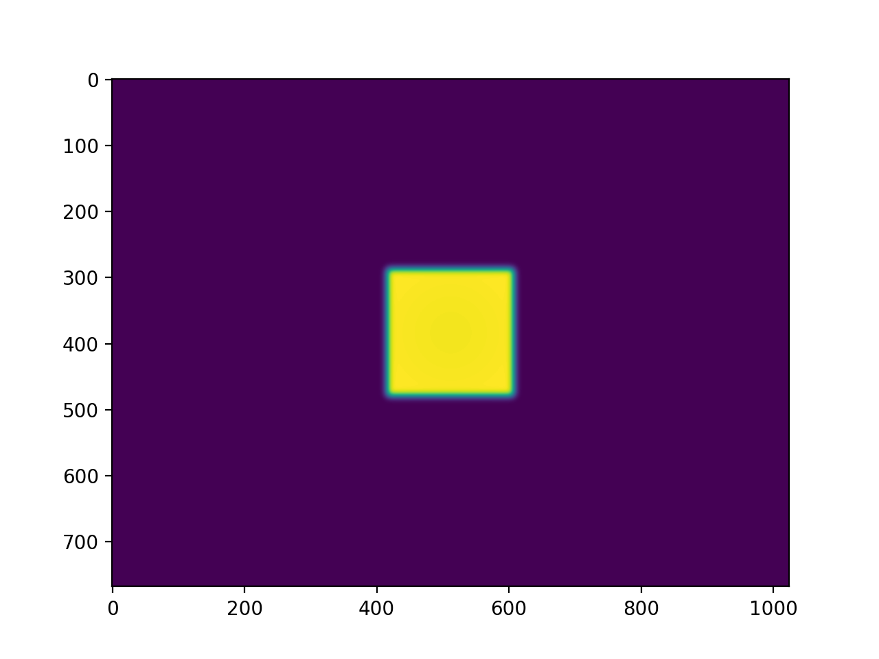
as1000 = AS1000Image() # this will set the pixel size and shape automatically
as1000.add_layer(FilteredFieldLayer(field_size_mm=(50, 50))) # create a 50x50mm square field
as1000.add_layer(GaussianFilterLayer(sigma_mm=2)) # add an image-wide gaussian to simulate penumbra/scatter
as1000.generate_dicom(file_out_name="my_AS1000.dcm", gantry_angle=45) # create a DICOM file with the simulated image
# plot the generated image
plt.imshow(as1000.image)
(Source code, png, hires.png, pdf)
Layers & Simulators
Layers are very simple structures. They usually have constructor arguments specific to the layer and always define an
apply method with the signature .apply(image, pixel_size) -> image. The apply method returns the modified image
(a numpy array). That’s it!
Simulators are also simple and define the parameters of the image to which layers are added. They have pixel_size
and shape properties and always have an add_layer method with the signature .add_layer(layer: Layer). They
also have a generate_dicom method for dumping the image along with mostly stock metadata to DICOM.
Extending Layers & Simulators
This module was meant to be extensible. That’s why the structures are defined so simply. To create a custom simulator,
inherit from Simulator and define the pixel size and shape. Note that generating DICOM does not come for free:
from pylinac.core.image_generator.simulators import Simulator

class AS5000(Simulator):
    pixel_size = 0.12
    shape = (5000, 5000)

# use like any other simulator
To implement a custom layer, inherit from Layer and implement the apply method:
from pylinac.core.image_generator.layers import Layer

class MyAwesomeLayer(Layer):

    def apply(image, pixel_size):
        # do stuff here
        return image

# use
from pylinac.core.image_generator import AS1000Image

as1000 = AS1000Image()
as1000.add_layer(MyAwesomeLayer())
...
Examples
Let’s make some images!
Simple Open Field
from matplotlib import pyplot as plt
from pylinac.core.image_generator import AS1000Image
from pylinac.core.image_generator.layers import FilteredFieldLayer, GaussianFilterLayer
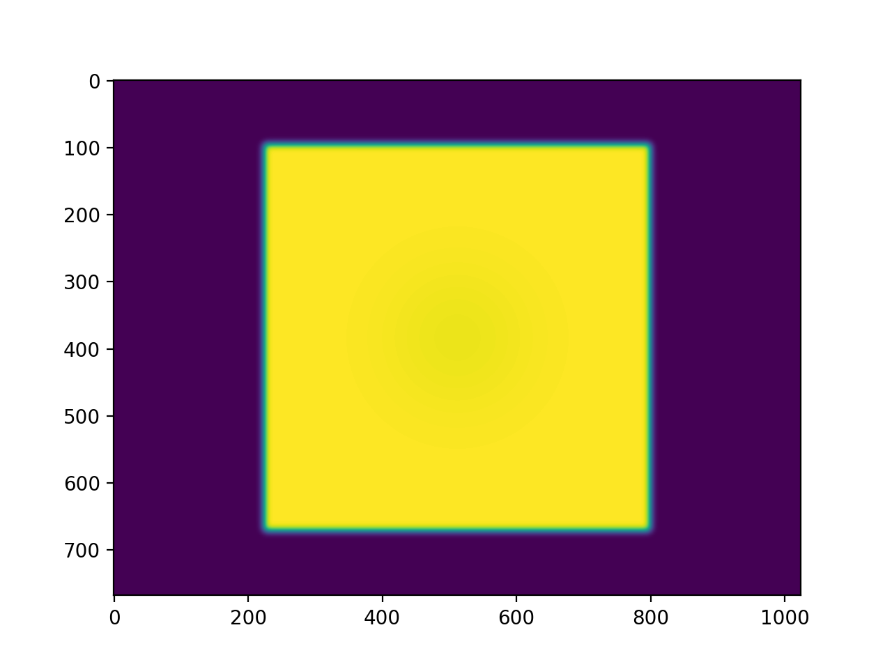
as1000 = AS1000Image() # this will set the pixel size and shape automatically
as1000.add_layer(FilteredFieldLayer(field_size_mm=(150, 150))) # create a 50x50mm square field
as1000.add_layer(GaussianFilterLayer(sigma_mm=2)) # add an image-wide gaussian to simulate penumbra/scatter
# plot the generated image
plt.imshow(as1000.image)
(Source code, png, hires.png, pdf)
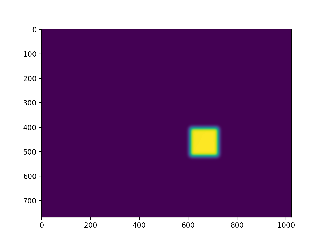
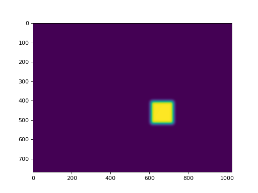
Off-center Open Field
from matplotlib import pyplot as plt
from pylinac.core.image_generator import AS1000Image
from pylinac.core.image_generator.layers import FilteredFieldLayer, GaussianFilterLayer

as1000 = AS1000Image()  # this will set the pixel size and shape automatically
as1000.add_layer(FilteredFieldLayer(field_size_mm=(30, 30), cax_offset_mm=(20, 40)))
as1000.add_layer(GaussianFilterLayer(sigma_mm=3))
# plot the generated image
plt.imshow(as1000.image)
(Source code, png, hires.png, pdf)
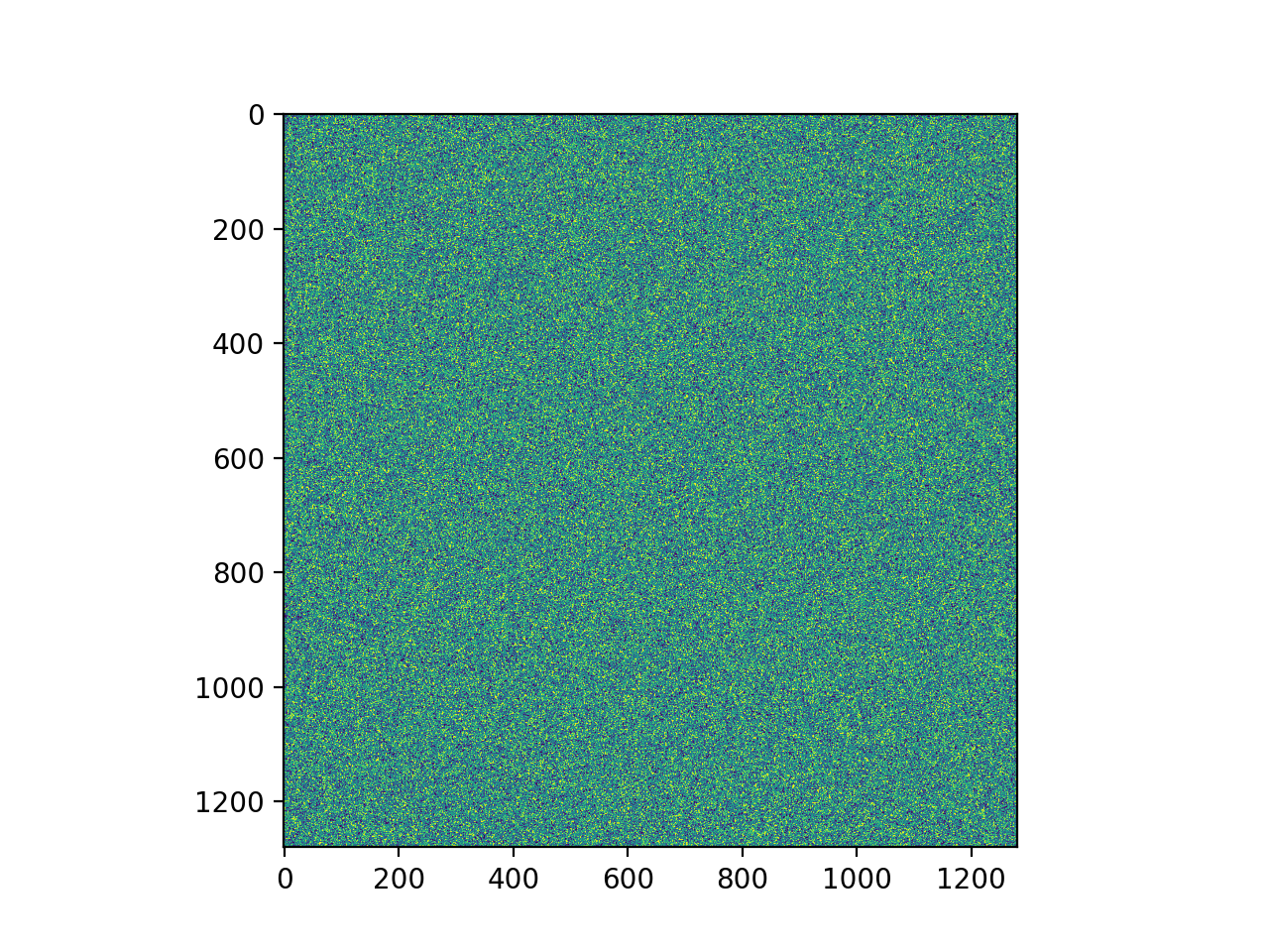
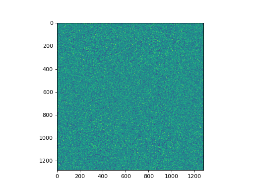
Winston-Lutz FFF Cone Field with Noise
from matplotlib import pyplot as plt
from pylinac.core.image_generator import AS1200Image
from pylinac.core.image_generator.layers import FilterFreeConeLayer, GaussianFilterLayer, PerfectBBLayer, RandomNoiseLayer

as1200 = AS1200Image()
as1200.add_layer(FilterFreeConeLayer(50))
as1200.add_layer(PerfectBBLayer(bb_size_mm=5))
as1200.add_layer(GaussianFilterLayer(sigma_mm=2))
as1200.add_layer(RandomNoiseLayer(sigma=2000))
# plot the generated image
plt.imshow(as1200.image)
(Source code, png, hires.png, pdf)
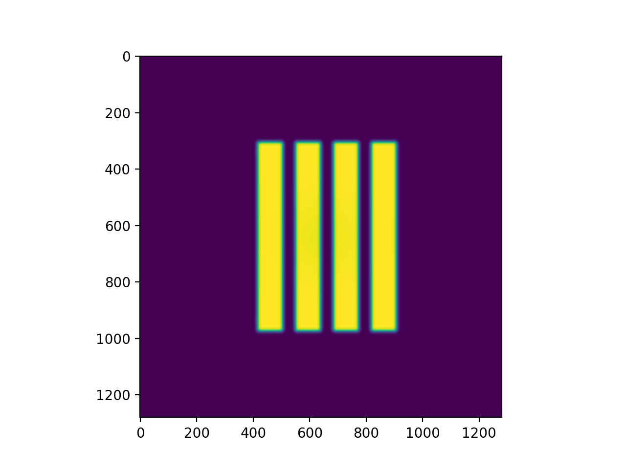
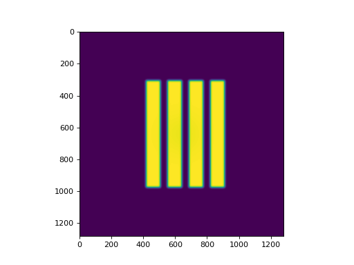
VMAT DRMLC
from matplotlib import pyplot as plt
from pylinac.core.image_generator import AS1200Image
from pylinac.core.image_generator.layers import FilteredFieldLayer, GaussianFilterLayer

as1200 = AS1200Image()
as1200.add_layer(FilteredFieldLayer((150, 20), cax_offset_mm=(0, -40)))
as1200.add_layer(FilteredFieldLayer((150, 20), cax_offset_mm=(0, -10)))
as1200.add_layer(FilteredFieldLayer((150, 20), cax_offset_mm=(0, 20)))
as1200.add_layer(FilteredFieldLayer((150, 20), cax_offset_mm=(0, 50)))
as1200.add_layer(GaussianFilterLayer())
plt.imshow(as1200.image)
plt.show()
(Source code, png, hires.png, pdf)
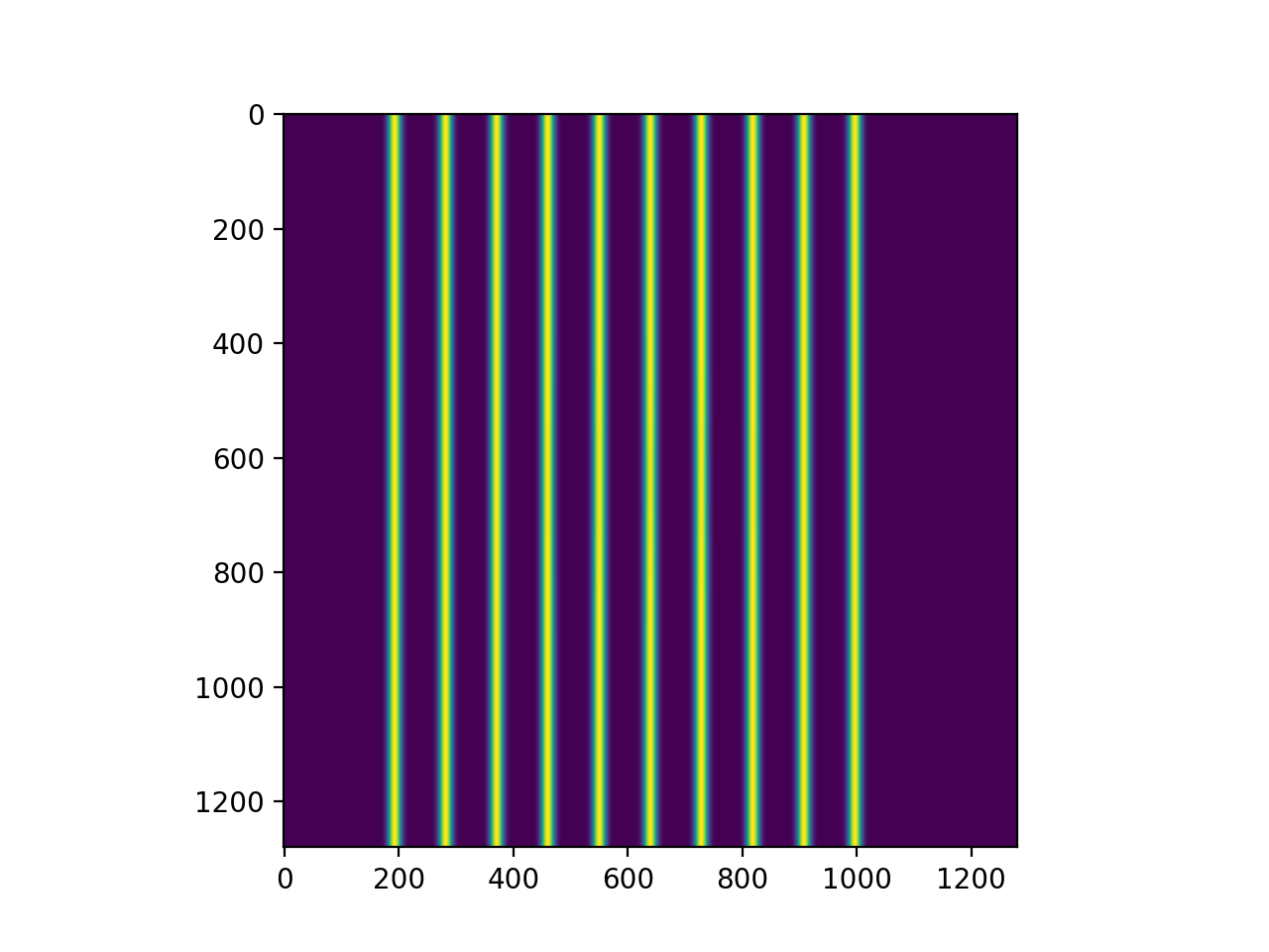
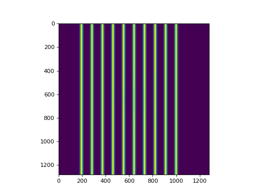
Picket Fence
from matplotlib import pyplot as plt
from pylinac.core.image_generator import AS1200Image
from pylinac.core.image_generator.layers import FilteredFieldLayer, GaussianFilterLayer

as1200 = AS1200Image()
height = 350
width = 4
offsets = range(-100, 100, 20)
for offset in offsets:
    as1200.add_layer(FilteredFieldLayer((height, width), cax_offset_mm=(0, offset)))
as1200.add_layer(GaussianFilterLayer())
plt.imshow(as1200.image)
plt.show()
(Source code, png, hires.png, pdf)
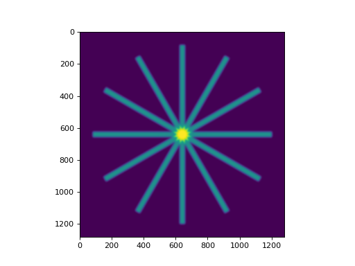
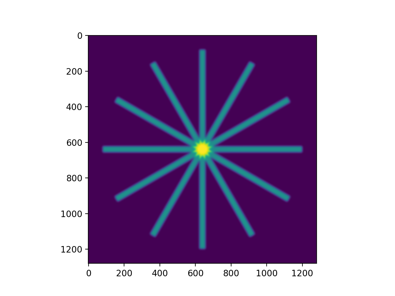
Starshot
Simulating a starshot requires a small trick as angled fields cannot be handled by default. The following example rotates the image after every layer is applied.
Note
Rotating the image like this is a convenient trick but note that it will rotate the entire existing image including all previous layers. This will also possibly erroneously adjust the horn effect simulation. Use with caution.
from scipy import ndimage
from matplotlib import pyplot as plt
from pylinac.core.image_generator import AS1200Image
from pylinac.core.image_generator.layers import FilteredFieldLayer, GaussianFilterLayer

as1200 = AS1200Image()
as1200.add_layer(FilteredFieldLayer((250, 7), alpha=0.5))
as1200.image = ndimage.rotate(as1200.image, 30, reshape=False, mode='nearest')
as1200.add_layer(FilteredFieldLayer((250, 7), alpha=0.5))
as1200.image = ndimage.rotate(as1200.image, 30, reshape=False, mode='nearest')
as1200.add_layer(FilteredFieldLayer((250, 7), alpha=0.5))
as1200.image = ndimage.rotate(as1200.image, 30, reshape=False, mode='nearest')
as1200.add_layer(FilteredFieldLayer((250, 7), alpha=0.5))
as1200.image = ndimage.rotate(as1200.image, 30, reshape=False, mode='nearest')
as1200.add_layer(FilteredFieldLayer((250, 7), alpha=0.5))
as1200.image = ndimage.rotate(as1200.image, 30, reshape=False, mode='nearest')
as1200.add_layer(FilteredFieldLayer((250, 7), alpha=0.5))
as1200.add_layer(GaussianFilterLayer())
plt.imshow(as1200.image)
plt.show()
(Source code, png, hires.png, pdf)

Helper utilities
Using the new utility functions of v2.5+ we can construct full dicom files of picket fence and winston-lutz sets of images:
from pylinac.core.image_generator import generate_picketfence, generate_winstonlutz
from pylinac.core import image_generator

sim = image_generator.simulators.AS1000Image()
field_layer = image_generator.layers.FilteredFieldLayer  # could also do FilterFreeLayer
generate_picketfence(simulator=Simulator, field_layer=FilteredFieldLayer,
                     file_out='pf_image.dcm',
                     pickets=11, picket_spacing_mm=20, picket_width_mm=2,
                     picket_height_mm=300, gantry_angle=0)
# we now have a pf image saved as 'pf_image.dcm'

# create a set of WL images
# this will create 4 images (via image_axes len) with an offset of 3mm to the left
# the function is smart enough to correct for the offset w/r/t gantry angle.
generate_winstonlutz(simulator=sim, field_layer=field_layer,
                     final_layers=[GaussianFilterLayer()], gantry_tilt=0,
                     dir_out='./wl_dir', offset_mm_left=3,
                     image_axes=[[0, 0, 0], [180, 0, 0], [90, 0, 0], [270, 0, 0]])
Tips & Tricks
- The
FilteredFieldLayerandFilterFree<Field, Cone>Layerhave gaussian filters applied to create a first-order approximation of the horn(s) of the beam. It doesn’t claim to be super-accurate, it’s just to give some reality to the images. You can adjust the magnitude of these parameters to simulate other energies (e.g. sharper horns) when defining the layer. - The
Perfect...Layers do not apply any energy correction as above. - Use
alphato adjust the intensity of the layer. E.g. the BB layer has a default alpha of -0.5 to simulate attenuation. This will subtract out up to half of the possible dose range existing on the image thus far (e.g. an open image of alpha 1.0 will be reduced to 0.5 after a BB is layered with alpha=-0.5). If you want to simulate a thick material like tungsten you can adjust the alpha to be lower (more attenuation). An alpha of 1 means full radiation, no attenuation (like an open field). - Generally speaking, don’t apply more than one
GaussianFilterLayersince they are additive. A good rule is to apply one filter at the end of your layering. - Apply
ConstantLayers at the beginning rather than the end.
Warning
Pylinac uses unsigned int16 datatypes (native EPID dtype). To keep images from flipping bits when adding layers,
pylinac will clip the values. Just be careful when, e.g. adding a ConstantLayer at the end of a layering. Better to do this
at the beginning.
API Documentation
Layers
-
class
pylinac.core.image_generator.layers.PerfectConeLayer(cone_size_mm: float = 10, cax_offset_mm: Tuple[float, float] = (0, 0), alpha: float = 1.0)[source]¶ Bases:
pylinac.core.image_generator.layers.LayerA cone without flattening filter effects
-
class
pylinac.core.image_generator.layers.FilterFreeConeLayer(cone_size_mm: float = 10, cax_offset_mm: Tuple[float, float] = (0, 0), alpha: float = 1.0, filter_magnitude: float = 0.4, filter_sigma_mm: float = 80, penumbra_mm: float = 2)[source]¶ Bases:
pylinac.core.image_generator.layers.PerfectConeLayerA cone with flattening filter effects.
-
class
pylinac.core.image_generator.layers.PerfectFieldLayer(field_size_mm: Tuple[float, float] = (10, 10), cax_offset_mm: Tuple[float, float] = (0, 0), alpha: float = 1.0)[source]¶ Bases:
pylinac.core.image_generator.layers.LayerA square field without flattening filter effects
-
class
pylinac.core.image_generator.layers.FilteredFieldLayer(field_size_mm: Tuple[float, float] = (10, 10), cax_offset_mm: Tuple[float, float] = (0, 0), alpha: float = 1.0, gaussian_height: float = 0.03, gaussian_sigma_mm: float = 32)[source]¶ Bases:
pylinac.core.image_generator.layers.PerfectFieldLayerA square field with flattening filter effects
-
class
pylinac.core.image_generator.layers.FilterFreeFieldLayer(field_size_mm: Tuple[float, float] = (10, 10), cax_offset_mm: Tuple[float, float] = (0, 0), alpha: float = 1.0, gaussian_height: float = 0.4, gaussian_sigma_mm: float = 80)[source]¶ Bases:
pylinac.core.image_generator.layers.FilteredFieldLayerA square field with flattening filter free (FFF) effects
-
class
pylinac.core.image_generator.layers.PerfectBBLayer(bb_size_mm: float = 5, cax_offset_mm: Tuple[float, float] = (0, 0), alpha: float = -0.5)[source]¶ Bases:
pylinac.core.image_generator.layers.PerfectConeLayerA BB-like layer. Like a cone, but with lower alpha (i.e. higher opacity)
-
apply(image: numpy.ndarray, pixel_size: float, mag_factor: float) → numpy.ndarray¶ Apply the layer. Takes a 2D array and pixel size value in and returns a modified array.
-
-
class
pylinac.core.image_generator.layers.GaussianFilterLayer(sigma_mm: float = 2)[source]¶ Bases:
pylinac.core.image_generator.layers.LayerA Gaussian filter. Simulates the effects of scatter on the field
-
class
pylinac.core.image_generator.layers.RandomNoiseLayer(mean: float = 0.0, sigma: float = 0.01)[source]¶ Bases:
pylinac.core.image_generator.layers.LayerA salt and pepper noise, simulating dark current
Simulators
-
class
pylinac.core.image_generator.simulators.AS500Image(sid: float = 1500)[source]¶ Bases:
pylinac.core.image_generator.simulators.SimulatorSimulates an AS500 EPID image.
Parameters: sid – Source to image distance in mm. -
generate_dicom(file_out_name: str, gantry_angle: float = 0.0, coll_angle: float = 0.0, table_angle: float = 0.0) → None[source]¶ Generate a DICOM file with the constructed image (via add_layer)
-
add_layer(layer: pylinac.core.image_generator.layers.Layer) → None¶ Add a layer to the image
-
-
class
pylinac.core.image_generator.simulators.AS1000Image(sid: float = 1500)[source]¶ Bases:
pylinac.core.image_generator.simulators.SimulatorSimulates an AS1000 EPID image.
Parameters: sid – Source to image distance in mm. -
generate_dicom(file_out_name: str, gantry_angle: float = 0.0, coll_angle: float = 0.0, table_angle: float = 0.0) → None[source]¶ Generate a DICOM file with the constructed image (via add_layer)
-
add_layer(layer: pylinac.core.image_generator.layers.Layer) → None¶ Add a layer to the image
-
-
class
pylinac.core.image_generator.simulators.AS1200Image(sid: float = 1500)[source]¶ Bases:
pylinac.core.image_generator.simulators.SimulatorSimulates an AS1200 EPID image.
Parameters: sid – Source to image distance in mm. -
generate_dicom(file_out_name: str, gantry_angle: float = 0.0, coll_angle: float = 0.0, table_angle: float = 0.0) → None[source]¶ Generate a DICOM file with the constructed image (via add_layer)
-
add_layer(layer: pylinac.core.image_generator.layers.Layer) → None¶ Add a layer to the image
-
Helpers
-
pylinac.core.image_generator.utils.generate_picketfence(simulator: pylinac.core.image_generator.simulators.Simulator, field_layer: Union[pylinac.core.image_generator.layers.FilterFreeFieldLayer, pylinac.core.image_generator.layers.FilteredFieldLayer], file_out: str, final_layers: List[pylinac.core.image_generator.layers.Layer] = None, pickets: int = 11, picket_spacing_mm: float = 20, picket_width_mm: int = 2, picket_height_mm=300, gantry_angle=0) → None[source]¶ Create a mock picket fence image. Will always be up-down.
Parameters: - simulator – The image simulator
- field_layer – The primary field layer
- file_out – The name of the file to save the DICOM file to.
- final_layers – Optional layers to apply at the end of the procedure. Useful for noise or blurring.
- pickets – The number of pickets
- picket_spacing_mm – The space between pickets
- picket_width_mm – Picket width parallel to leaf motion
- picket_height_mm – Picket height parallel to leaf motion
- gantry_angle – Gantry angle; sets the DICOM tag.
-
pylinac.core.image_generator.utils.generate_winstonlutz(simulator: pylinac.core.image_generator.simulators.Simulator, field_layer: Type[pylinac.core.image_generator.layers.Layer], dir_out: str, field_size_mm: Tuple[float, float] = (30, 30), final_layers: Optional[List[pylinac.core.image_generator.layers.Layer]] = None, bb_size_mm: float = 5, offset_mm_left: float = 0, offset_mm_up: float = 0, offset_mm_in: float = 0, image_axes: List[Tuple[int, int, int]] = [(0, 0, 0), (90, 0, 0), (180, 0, 0), (270, 0, 0)], gantry_tilt: float = 0, gantry_sag: float = 0, clean_dir: bool = True) → List[str][source]¶ Create a mock set of WL images, simulating gantry sag effects. Produces one image for each item in image_axes.
Parameters: - simulator – The image simulator
- field_layer – The primary field layer simulating radiation
- dir_out – The directory to save the images to.
- field_size_mm – The field size of the radiation field in mm
- final_layers – Layers to apply after generating the primary field and BB layer. Useful for blurring or adding noise.
- bb_size_mm – The size of the BB. Must be positive.
- offset_mm_left – How far left (lat) to set the BB. Can be positive or negative.
- offset_mm_up – How far up (vert) to set the BB. Can be positive or negative.
- offset_mm_in – How far in (long) to set the BB. Can be positive or negative.
- image_axes – List of axis values for the images. Sequence is (Gantry, Coll, Couch).
- gantry_tilt – The tilt of the gantry that affects the position at 0 and 180. Simulates a simple cosine function.
- gantry_sag – The sag of the gantry that affects the position at gantry=90 and 270. Simulates a simple sine function.
- clean_dir – Whether to clean out the output directory. Useful when iterating.
-
pylinac.core.image_generator.utils.generate_winstonlutz_cone(simulator: pylinac.core.image_generator.simulators.Simulator, cone_layer: Union[Type[pylinac.core.image_generator.layers.FilterFreeConeLayer], Type[pylinac.core.image_generator.layers.PerfectConeLayer]], dir_out: str, cone_size_mm: float = 17.5, final_layers: Optional[List[pylinac.core.image_generator.layers.Layer]] = None, bb_size_mm: float = 5, offset_mm_left: float = 0, offset_mm_up: float = 0, offset_mm_in: float = 0, image_axes: List[Tuple[int, int, int]] = [(0, 0, 0), (90, 0, 0), (180, 0, 0), (270, 0, 0)], gantry_tilt: float = 0, gantry_sag: float = 0, clean_dir: bool = True) → List[str][source]¶ Create a mock set of WL images with a cone field, simulating gantry sag effects. Produces one image for each item in image_axes.
Parameters: - simulator – The image simulator
- cone_layer – The primary field layer simulating radiation
- dir_out – The directory to save the images to.
- cone_size_mm – The field size of the radiation field in mm
- final_layers – Layers to apply after generating the primary field and BB layer. Useful for blurring or adding noise.
- bb_size_mm – The size of the BB. Must be positive.
- offset_mm_left – How far left (lat) to set the BB. Can be positive or negative.
- offset_mm_up – How far up (vert) to set the BB. Can be positive or negative.
- offset_mm_in – How far in (long) to set the BB. Can be positive or negative.
- image_axes – List of axis values for the images. Sequence is (Gantry, Coll, Couch).
- gantry_tilt – The tilt of the gantry that affects the position at 0 and 180. Simulates a simple cosine function.
- gantry_sag – The sag of the gantry that affects the position at gantry=90 and 270. Simulates a simple sine function.
- clean_dir – Whether to clean out the output directory. Useful when iterating.