Field Analysis¶

Overview¶

The field analysis module (pylinac.field_analysis) allows a physicist to analyze metrics from an EPID or 2D device array to measure penumbra, field width, etc. Additionally, protocols can be used which can calculate flatness & symmetry. The module is very flexible, allowing users to choose different types of interpolation, normalization, centering, etc. Users can also creat custom protocols to perform other types of field analysis within the main pylinac flow.

The module implements traditional analysis like FWHM as well as new methods as outlined in the pre-publication of the NCS-33 report which include edge fitting for FFF fields as well as a “top” calculation for the center position of FFF beams.

Note

This is not a purely faithful implementation of NCS-33. There are a few differences w/r/t how stringent field widths are applied. E.g. the “top” calculation in NCS-33 is over the central 5cm. Pylinac simply uses a field width ratio which may or may not be 5cm.

The module contains two main classes FieldAnalysis which is used for EPID images and DeviceFieldAnalysis which is used for 2D device arrays.

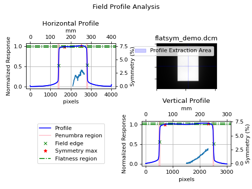
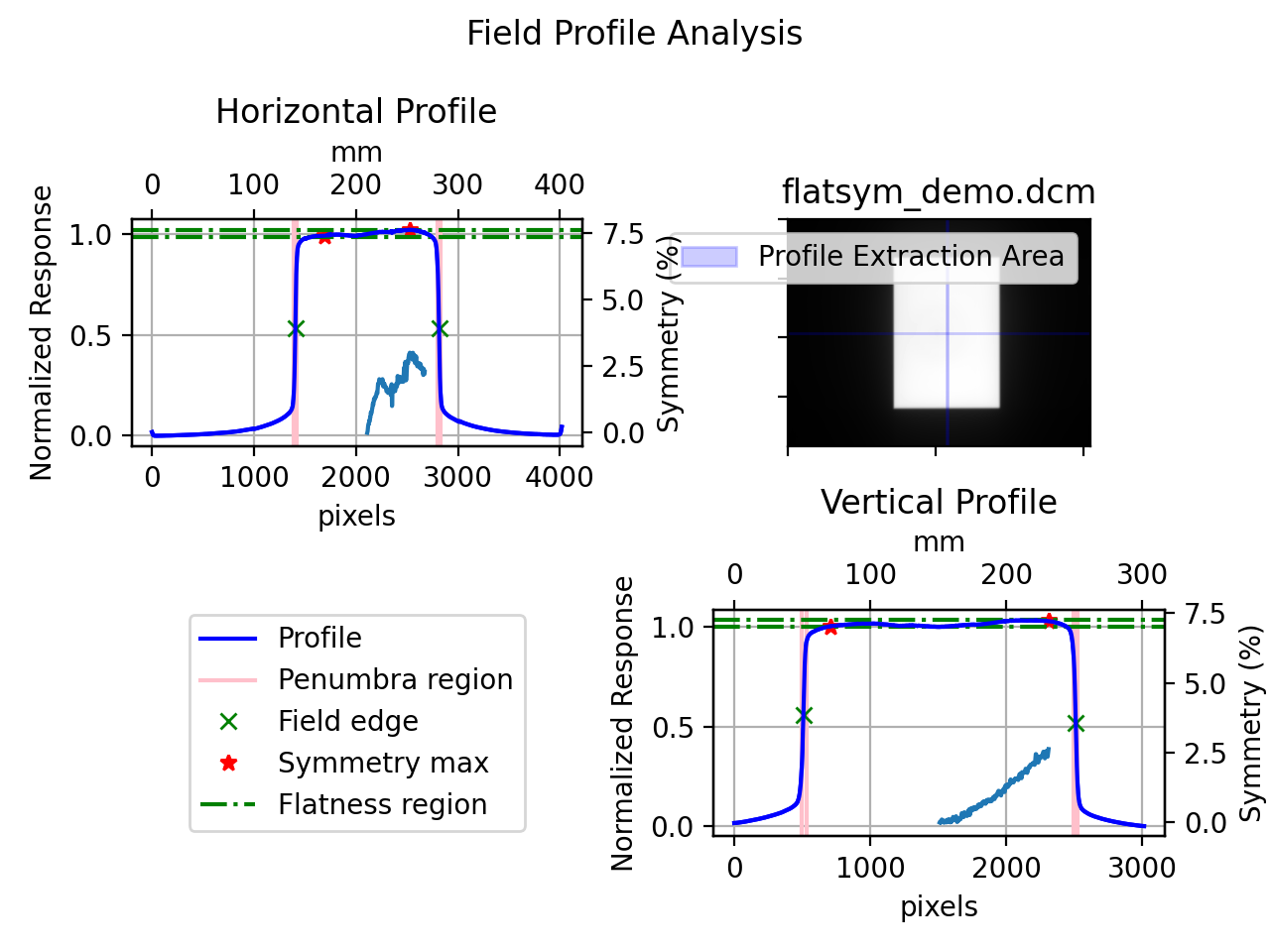
Running the Demo¶

To run the demo, import the main class and run the demo method:

from pylinac import FieldAnalysis

FieldAnalysis.run_demo()

(Source code, png, hires.png, pdf)

Which will also result in the following output:

Field Analysis Results
----------------------
File: E:\OneDrive - F...demo_files\flatsym_demo.dcm
Protocol: VARIAN
Centering method: Beam center
Normalization method: Beam center
Interpolation: Linear
Edge detection method: Inflection Derivative

Penumbra width (20/80):
Left: 2.7mm
Right: 3.0mm
Top: 3.9mm
Bottom: 2.8mm

Field Size:
Horizontal: 140.9mm
Vertical: 200.3mm

CAX to edge distances:
CAX -> Top edge: 99.8mm
CAX -> Bottom edge: 100.5mm
CAX -> Left edge: 60.4mm
CAX -> Right edge: 80.5mm

Top slope: -0.006%/mm
Bottom slope: 0.044%/mm
Left slope: 0.013%/mm
Right slope: 0.014%/mm

Protocol data:
--------------
Vertical symmetry: -2.631%
Horizontal symmetry: -3.006%

Vertical flatness: 1.700%
Horizontal flatness: 1.857%

Typical Use¶

In most instances, a physicist is interested in quickly calculating the flatness, symmetry, or both of the image in question. The field_analysis module allows you to do this easily and quickly.

To get started, import the FieldAnalysis class:

from pylinac import FieldAnalysis

Loading images is easy and just like any other module:

# from a file
my_file = r"C:/my/QA/folder/img.dcm"
my_img = FieldAnalysis(path=my_file)

Alternatively, you can load data from a 2D device array:

from pylinac import DeviceFieldAnalysis

# Profiler file
my_file = r"C:/my/profiler/data.prm"
my_img = DeviceFieldAnalysis(path=my_file)

If you don’t have an image you can load the demo image:

my_img = FieldAnalysis.from_demo_image()

You can then calculate several field metrics with the analyze() method:

my_img.analyze()

After analysis, the results can be printed, plotted, or saved to a PDF:

print(my_img.results())  # print results as a string
my_img.plot_analyzed_image()  # matplotlib image
my_img.publish_pdf(filename="flatsym.pdf")  # create PDF and save to file
my_img.results_data()  # dict of results

Analyze Options¶

The analysis algorithm allows the user to change numerous parameters about the analysis including automatic/manual centering, profile extraction width, field width ratio, penumbra values, interpolation, normalization, and edge detection. See pylinac.field_analysis.FieldAnalysis.analyze() for details on each parameter

The protocol can also be specified here; this is where both default and custom algorithms like flatness and symmetry can be used. See Protocol Definitions for the common flatness/symmetry algorithms provided out of the box. For custom protocols, see Creating & Using Custom Protocols.

from pylinac import Protocol, Centering, Edge, Normalization, Interpolation

my_img.analyze(protocol=Protocol.ELEKTA, centering=Centering.BEAM_CENTER, in_field_ratio=0.8,
               is_FFF=True, interpolation=Interpolation.SPLINE, interpolation_resolution_mm=0.2,
               edge_detection_method=Edge.INFLECTION_HILL)

Centering¶

There are 3 centering options: manual, beam center, and geometric center.

Manual¶

Manual centering means that you as the user specify the position of the image that the profiles are taken from.

from pylinac import FieldAnalysis, Centering

fa = FieldAnalysis(...)
fa.analyze(..., centering=Centering.MANUAL)  # default is the middle of the image

# or specify a custom location
fa.analyze(..., centering=Centering.MANUAL, vert_position=0.3, horiz_position=0.8)
# take profile at 30% width (i.e. left side) and 80% height

Beam center¶

This is the default for EPID images/FieldAnalysis. It first looks for the field to find the approximate center along each axis. Then it extracts the profiles and continues. This is helpful if you always want to be at the center of the field, even for offset fields or wedges.

from pylinac import FieldAnalysis, Centering

fa = FieldAnalysis(...)
fa.analyze(...)  # nothing special needed as it's the default

# You CANNOT specify a position. These values will be ignored
fa.analyze(..., centering=Centering.BEAM_CENTER, vert_position=0.3, horiz_position=0.8)
# this is allowed but will result in the same result as above

Geometric center¶

This is the default for 2D device arrays/DeviceFieldAnalysis. It will always find the middle pixel and extract the profiles from there. This is helpful if you always want to be at the center of the image.

from pylinac import FieldAnalysis, Centering

fa = FieldAnalysis(...)
fa.analyze(...)  # nothing special needed as it's the default

# You CANNOT specify a position. These values will be ignored
fa.analyze(..., centering=Centering.GEOMETRIC_CENTER, vert_position=0.3, horiz_position=0.8)
# this is allowed but will result in the same result as above

Edge detection¶

Edge detection is important for determining the field width and beam center (which is often used for symmetry). There are 3 detection strategies: FWHM, inflection via derivative, and inflection via the Hill/sigmoid/4PNLR function.

FWHM¶

The full-width half-max strategy is traditional and works for flat beams. It can give poor values for FFF beams.

from pylinac import FieldAnalysis, Edge

fa = FieldAnalysis(...)
fa.analyze(..., edge_detection_method=Edge.FWHM)

Inflection (derivative)¶

The inflection point via the derivative is useful for both flat and FFF beams, and is thus the default for FieldAnalysis. The method will find the positions of the max and min derivative of the values. Using a 0-crossing of the 2nd derivative can be tripped up by noise so it is not used.

Note

This method is recommended for high spatial resolution images such as the EPID, where the derivative has several points to use at the beam edge. It is not recommended for 2D device arrays.

from pylinac import FieldAnalysis, Edge

fa = FieldAnalysis(...) # nothing special needed as it's the default

# you may also specify the edge smoothing value. This is a gaussian filter applied to the derivative just for the purposes of finding the min/max derivative.
# This is to ensure the derivative is not caught by some noise. It is usually not necessary to change this.
fa = FieldAnalysis(..., edge_smoothing_ratio=0.005)

Inflection (Hill)¶

The inflection point via the Hill function is useful for both flat and FFF beams The fitting of the function is best for low-resolution data, and is thus the default for DeviceFieldAnalysis. The Hill function, the sigmoid function, and 4-point non-linear regression belong to a family of logistic equations to fit a dual-curved value. Since these fit a function to the data the resolution problems are eliminated. Some examples can be seen here. The generalized logistic function has helpful visuals as well here.

The function used here is:

\(f(x) = A + \frac{B - A}{1 + \frac{C}{x}^D}\)

where \(A\) is the low asymptote value (~0 on the left edge of a field), \(B\) is the high asymptote value (~1 for a normalized beam on the left edge), \(C\) is the inflection point of the sigmoid curve, and \(D\) is the slope of the sigmoid.

The function is fitted to the edge data of the field on each side to return the function. From there, the inflection point, penumbra, and slope can be found.

Note

This method is recommended for low spatial resolution images such as 2D device arrays, where there is very little data at the beam edges. While it can be used for EPID images as well, the fit can have small errors as compared to the direct data. The fit, however, is much better than a linear or even spline interpolation at low resolutions.

from pylinac import FieldAnalysis, Edge

fa = FieldAnalysis(..., edge_detection_method=Edge.INFLECTION_HILL)

# you may also specify the hill window. This is the size of the window (as a ratio) to use to fit the field edge to the Hill function.
fa = FieldAnalysis(..., edge_detection_method=Edge.INFLECTION_HILL, hill_window_ratio=0.05)
# i.e. use a 5% field width about the edges to fit the Hill function.

Note

When using this method, the fitted Hill function will also be plotted on the image. Further, the exact field edge marker (green x) may not align with the Hill function fit. This is just a rounding issue due to the plotting mechanism. The field edge is really using the Hill fit under the hood.

Normalization¶

There are 4 options for interpolation: None, GEOMETRIC_CENTER, BEAM_CENTER, and MAX. These should be self-explanatory, especially in light of the centering explanations.

from pylinac import FieldAnalysis, Normalization

fa = FieldAnalysis(...)
fa.analyze(..., normalization_method=Normalization.BEAM_CENTER)

Interpolation¶

There are 3 options for interpolation: NONE, LINEAR, and SPLINE.

None¶

A method of NONE will obviously apply no interpolation. Other interpolation parameters (see below) are ignored. This is the default method for DeviceFieldAnalysis

Note

When plotting the data, if interpolation is None and the data is from a device, the data will be plotted as individual markers (+). If interpolation is applied to device data or it is a DICOM/EPID image, the data is plotted as a line.

Linear¶

This will apply a linear interpolation to the original data. Along with this, the parameter interpolation_resolution_mm determine the amount of interpolation. E.g. a value of 0.1 will resample the data to get data points 0.1mm apart. This is the default method for FieldAnalysis.

from pylinac import FieldAnalysis, Interpolation

fa = FieldAnalysis(...)
fa.analyze(..., interpolation=Interpolation.LINEAR, interpolation_resolution_mm=0.1)

Spline¶

This will apply a cubic spline interpolation to the original data. Along with this, the parameter interpolation_resolution_mm determine the amount of interpolation. E.g. a value of 0.1 will resample the data to get data points 0.1mm apart.

from pylinac import FieldAnalysis, Interpolation

fa = FieldAnalysis(...)
fa.analyze(..., interpolation=Interpolation.SPLINE, interpolation_resolution_mm=0.1)

Protocol Definitions¶

There are multiple definitions for both flatness and symmetry. Your machine vendor uses certain equations, or your clinic may use a specific definition. Pylinac has a number of built-in definitions which you can use. Know also that you can create your own if you don’t like/want to extend these Creating & Using Custom Protocols.

None¶

Technically, you are allowed a “None” protocol (Protocol.NONE), which just means nothing beyond the basic field analysis is performed. If you just want the penumbra, distances to CAX, etc, without flatness/symmetry/custom algos then this is for you.

Varian¶

This is the default protocol if you don’t specify one (Protocol.VARIAN). Two metrics are included, flatness & symmetry.

from pylinac import FieldAnalysis, Protocol

fa = FieldAnalysis(...)
fa.analyze(protocol=Protocol.VARIAN, ...)
...

Flatness¶

Flatness is defined by the variation (difference) across the field values within the field width.

\(flatness = 100 * |D_{max} - D_{min}| / (D_{max} + D_{min})\)

If the field width is set to, e.g. 80%, then the flatness is calculated over all the values within that 80%. Flatness is a scalar and always positive.

Symmetry¶

Symmetry is defined as the Point Difference:

\(symmetry = 100 * max(|L_{pt} - R_{pt}|)/ D_{CAX}\)

where \(L_{pt}\) and \(R_{pt}\) are equidistant from the beam center.

Symmetry is calculated over the specified field width (e.g. 80%) as set in by analyze(). Symmetry can be positive or negative. A negative value means the right side is higher. A positive value means the left side is higher.

Elekta¶

This is specified by passing protocol=Protocol.ELEKTA to analyze.

from pylinac import FieldAnalysis, Protocol

fa = FieldAnalysis(...)
fa.analyze(protocol=Protocol.ELEKTA, ...)
...

Flatness¶

Flatness is defined by the ratio of max/min across the field values within the field width.

\(flatness = 100 * D_{max}/D_{min}\)

If the field width is set to, e.g. 80%, then the flatness is calculated over all the values within that 80%. Flatness is a scalar and always positive.

Symmetry¶

Symmetry is defined as the Point Difference Quotient (aka IEC):

\(symmetry = 100 * max(|L_{pt}/R_{pt}|, |R_{pt}/L_{pt}|)\)

where \(L_{pt}\) and \(R_{pt}\) are equidistant from the beam center.

Symmetry is calculated over the specified field width (e.g. 80%) as set in by analyze(). Symmetry can be positive or negative. A negative value means the right side is higher. A positive value means the left side is higher.

Siemens¶

This is specified by passing protocol=Protocol.SIEMENS to analyze.

from pylinac import FieldAnalysis, Protocol

fa = FieldAnalysis(...)
fa.analyze(protocol=Protocol.SIEMENS, ...)
...

Flatness¶

Flatness is defined by the variation (difference) across the field values within the field width.

\(flatness = 100 * |D_{max} - D_{min}| / (D_{max} + D_{min})\)

If the field width is set to, e.g. 80%, then the flatness is calculated over all the values within that 80%. Flatness is a scalar and always positive.

Symmetry¶

Symmetry is defined as the ratio of area on each side about the CAX:

\(symmetry = 100 * (A_{left} - A_{right}) / (A_{left} + A_{right})\)

Symmetry is calculated over the specified field width (e.g. 80%) as set in by analyze(). Symmetry can be positive or negative. A negative value means the right side is higher. A positive value means the left side is higher.

Creating & Using Custom Protocols¶

Protocols allow the user to perform specific image metric algorithms. This includes things like flatness & symmetry. Depending on the protocol, different methods of determining the flatness/symmetry/whatever exist. Pylinac provides a handful of protocols out of the box, but it is easy to add your own custom algorithms.

To create a custom protocol you must 1) create custom algorithm functions, 2) create a protocol class that 3) inherits from Enum and 4) defines a dictionary with a calc, unit, and plot key/value pair. The plot key is optional; it allows you to plot something if you also want to see your special algorithm (e.g. if it used a fitting function and you want to plot the fitted values).

calc should be a function to calculate a specific, singular value such as flatness.
unit should be a string that specifies the unit of calc. If it is unitless leave it as an empty string ('')
plot is OPTIONAL and is a function that can plot something to the profile views (e.g. a fitting function)

The calc and plot values should be functions with a specific signature as shown in the example below:

import enum

# create the custom algorithm functions
# the ``calc`` function must have the following signature
def my_special_flatness(profile: SingleProfile, in_field_ratio: float, **kwargs) -> float:
    # do whatever. Must return a float. ``profile`` will be called twice, once for the vertical profile and horizontal profile.
    # the kwargs are passed to ``analyze`` and can be used here for your own purposes (e.g. fitting parameters)
    my_special_value = kwargs.get("funkilicious")
    flatness = profile...
    return flatness

# custom plot function for the above flatness function
# This is OPTIONAL
# If you do implement this, it must have the following signature
def my_special_flatness_plot(instance, profile: SingleProfile, axis: plt.Axes) -> None:
    # instance is the FieldAnalysis instance; i.e. it's basically ``self``.
    # do whatever; typically, you will do an axis.plot()
    axis.plot(...)

# custom protocol MUST inherit from Enum
class MySpecialProtocols(enum.Enum):
    # note you can specify several protocols if you wish
    PROTOCOL_1 = {
        # for each protocol, you can specify any number of metrics to calculate. E.g. 2 symmetry calculations
        'my flatness': {'calc': my_special_flatness, 'unit': '%', 'plot': my_special_flatness_plot},
        'my symmetry': ...,
        'my other flatness metric': ...,
    }
    PROTOCOL_2 = ...

# proceed as normal
fa = FieldAnalysis(...)
fa.analyze(protocol=MySpecialProtocols.PROTOCOL_1, ...)
...

Passing in custom parameters¶

You may pass custom parameters to these custom algorithms via the analyze method as simple keyword arguments:

fa = FieldAnalysis(...)
fa.analyze(..., my_special_variable=42)

The parameter will then be passed to the custom functions:

def my_special_flatness(profile: SingleProfile, in_field_ratio: float, **kwargs) -> float:
    my_special_value = kwargs.get("my_special_variable")  # 42
    flatness = profile...
    return flatness

Note

The SingleProfile passed to the functions is very powerful and can calculate numerous helpful data for you such as the field edges, minimum/maximum value within the field, and much more. Read the SingleProfile documentation before creating a custom algorithm.

Loading Device Data¶

The field analysis module can load data from a 2D device array. Currently, only the SNC Profiler is supported, but this will expand over time. The DeviceFieldAnalysis class and associated Device class will handle the loading and parsing of the file as well as spatial resolution information.

To load a Profiler dataset:

from pylinac import DeviceFieldAnalysis, Device

fa = DeviceFieldAnalysis(path='my/path/to/6x.prs', device=Device.PROFILER)
# proceed as normal
fa.analyze(...)

Note

While largely the same as the FieldAnalysis class, the DeviceFieldAnalysis’s analyze signature is different. Specifically, you cannot pass a vert/horiz position or width (since it’s not an image) nor can you pass a centering option. The table below shows the differences. Any parameter not shown is the same between the two.

Default differences¶
parameter	FieldAnalysis	DeviceFieldAnalysis
vert_position	0.5	N/A
horiz_position	0.5	N/A
vert_width	0.5	N/A
horiz_width	0.5	N/A
centering	Beam center	N/A
interpolation	Linear	None
normalization_method	Beam center	Geometric center
edge_detection_method	Inflection derivative	Inflection Hill

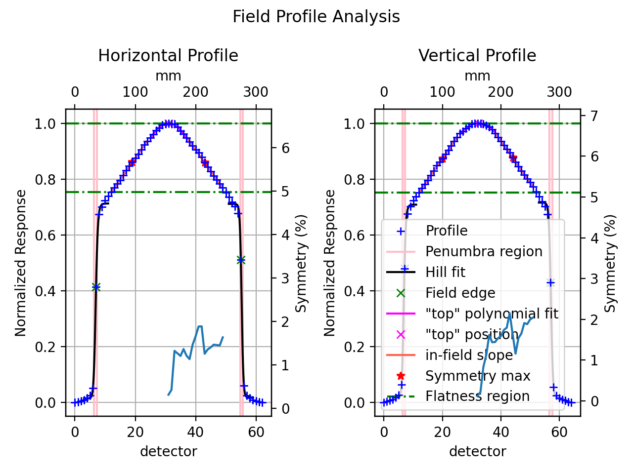
FFF fields¶

The field analysis module can handle FFF beams, or more specifically, calculating extra metrics associated with FFF fields. These metrics are largely from the NCS-33 pre-publication and include the “top” position, and the slopes of the field on each side.

These metrics are always calculated (even for flat beams), but will be shown in the results() output and also on the plotted image of plot_analyzed_image() if the is_FFF flag is true.

The easiest way to demonstrate this is through the Device demo, which is an FFF field:

from pylinac import DeviceFieldAnalysis, Protocol

fa = DeviceFieldAnalysis.from_demo_image()
fa.analyze(protocol=Protocol.VARIAN, is_FFF=True)
fa.plot_analyzed_image()

(Source code, png, hires.png, pdf)

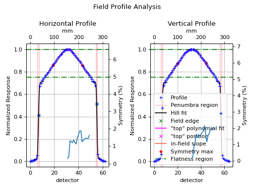
“Top” metric¶

The “top” metric is the fitted position of the peak of a FFF beam. It uses the central region of the field as specified by the slope_exclusion_ratio. E.g. if the value is 0.3 it will use the central 30% field width.

The central region is fitted to a 2nd order polynomial and then the max of the polynomial is found. That value is the “top” position. This helps to account for noise in the profile.

When printing results for an FFF beam there will be a section like so:

'Top' vertical distance from CAX: 1.3mm
'Top' horizontal distance from CAX: 0.6mm
'Top' vertical distance from beam center: 1.7mm
'Top' horizontal distance from beam center: 0.3mm

Field slope¶

For FFF beams, an additional metric is calculated: the slope of each side of the field. Since traditional flatness algorithms aren’t tuned for FFF beams they can be noisy or non-sensible. By measuring the slope of each side of the field the flatness can be measured more accurately (as a slope) for trending and consistency purposes.

The slope is calculated in the regions between the field width edges and the slope exclusion ratio. E.g. a field width ratio of 0.8 and a slope exclusion ratio of 0.4 will mean that the regions between +/-0.4 (0.8/2) from the CAX to +/-0.2 (0.4/2) will be used to fit linear regressions.

When printing results for an FFF beam there will be a section like so:

Top slope: 0.292%/mm
Bottom slope: -0.291%/mm
Left slope: 0.295%/mm
Right slope: -0.296%/mm

Accessing data¶

Changed in version 3.0.

Using the module in your own scripts? While the analysis results can be printed out, if you intend on using them elsewhere (e.g. in an API), they can be accessed the easiest by using the results_data() method which returns a FieldResult instance.

Note

While the pylinac tooling may change under the hood, this object should remain largely the same and/or expand. Thus, using this is more stable than accessing attrs directly.

You can access most data you get from results():

fa = FieldAnalysis… fa.analyze(…) data = fa.results_data()

data.top_penumbra_mm data.beam_center_to_left_mm

You may also access protocol data in the protocol_results dictionary. These results must be in a dictionary because the protocol names and fields are dynamic and not known a priori.

data.protocol_results[‘flatness_vertical’] data.protocol_results[‘symmetry_horizontal’]

The keys of this dict are defined by the protocol names. Using the example from the Creating & Using Custom Protocols section, we would access that custom protocol data as:

data.protocol_results[‘my flatness_vertical’] data.protocol_results[‘my flatness_horizontal’]

because the protocol name was my flatness.

Algorithm¶

There is little of a true “algorithm” in field_analysis other than analyzing profiles. Thus, this section is more terminology and notekeeping.

Allowances

The image can be any size.
The image can be EPID (actually just DICOM) or a 2D device array file.
The image can be either inversion (Radiation is dark or light).
The image can be off-center.

Restrictions

The module is only meant for photon analysis at the moment (there are sometimes different equations for electrons for the same definition name).
Analysis is limited to normal/parallel directions. Thus if the image is rotated there is no way to account for it other than rotating the image before analysis.

Analysis

Extract profiles - With the positions given, profiles are extracted and analyzed according to the method specified (see Protocol Definitions). For symmetry calculations that operate around the CAX, the CAX must first be determined, which is the center of the FWHM of the profile.

API Documentation¶

Main classes¶

These are the classes a typical user may interface with.

class pylinac.field_analysis.FieldAnalysis(path: Union[str, BinaryIO], filter: Optional[int] = None)[source]¶

Bases: object

Class for analyzing the various parameters of a radiation image, most commonly an open image from a linac.

Parameters:	path – The path to the image. filter – If None, no filter is applied. If an int, a median filter of size n pixels is applied. Generally, a good idea. Default is None for backwards compatibility.

image = None¶

vert_profile = None¶

horiz_profile = None¶

classmethod from_demo_image()[source]¶: Load the demo image into an instance.

static run_demo() → None[source]¶: Run the Field Analysis demo by loading the demo image, print results, and plot the profiles.

analyze(protocol: pylinac.field_analysis.Protocol = <Protocol.VARIAN: {'symmetry': {'calc': <function symmetry_point_difference>, 'unit': '%', 'plot': <function plot_symmetry_point_difference>}, 'flatness': {'calc': <function flatness_dose_difference>, 'unit': '%', 'plot': <function plot_flatness>}}>, centering: Union[pylinac.field_analysis.Centering, str] = <Centering.BEAM_CENTER: 'Beam center'>, vert_position: float = 0.5, horiz_position: float = 0.5, vert_width: float = 0, horiz_width: float = 0, in_field_ratio: float = 0.8, slope_exclusion_ratio: float = 0.2, invert: bool = False, is_FFF: bool = False, penumbra: Tuple[float, float] = (20, 80), interpolation: Union[pylinac.core.profile.Interpolation, str, None] = <Interpolation.LINEAR: 'Linear'>, interpolation_resolution_mm: float = 0.1, ground: bool = True, normalization_method: Union[pylinac.core.profile.Normalization, str] = <Normalization.BEAM_CENTER: 'Beam center'>, edge_detection_method: Union[pylinac.core.profile.Edge, str] = <Edge.INFLECTION_DERIVATIVE: 'Inflection Derivative'>, edge_smoothing_ratio: float = 0.003, hill_window_ratio: float = 0.15, **kwargs) → None[source]¶

Analyze the image to determine parameters such as field edges, penumbra, and/or flatness & symmetry.

Parameters:

protocol (Protocol) – The analysis protocol. See Protocol Definitions for equations.
centering (Centering) – The profile extraction position technique. Beam center will determine the beam center and take profiles through the middle. Geometric center will simply take profiles centered about the image in both axes. Manual will use the values of vert_position and horiz_position as the position. See Centering.
vert_position –
The distance ratio of the image to sample. E.g. at the default of 0.5 the profile is extracted in the middle of the image. 0.0 is at the left edge of the image and 1.0 is at the right edge of the image.

Note

This value only applies when centering is MANUAL.
horiz_position –
The distance ratio of the image to sample. E.g. at the default of 0.5 the profile is extracted in the middle of the image. 0.0 is at the top edge of the image and 1.0 is at the bottom edge of the image.

Note

This value only applies when centering is MANUAL.
vert_width – The width ratio of the image to sample. E.g. at the default of 0.0 a 1 pixel wide profile is extracted. 0.0 would be 1 pixel wide and 1.0 would be the vertical image width.
horiz_width – The width ratio of the image to sample. E.g. at the default of 0.0 a 1 pixel wide profile is extracted. 0.0 would be 1 pixel wide and 1.0 would be the horizontal image width.
in_field_ratio – The ratio of the field width to use for protocol values. E.g. 0.8 means use the 80% field width.
slope_exclusion_ratio –
This is the ratio of the field to use to 1) calculate the “top” of an FFF field as well as 2) exclude from the “slope” calculation of each side of the field. Alternatively, this also defines the area to use for the slope calculation. E.g. an in_field_ratio of 0.8 and slope_exclusion_ratio of 0.2 means the central 20% of the field is used to fit and calculate the “top”, while the region on either side of the central 20% between the central 80% is used to calculate a slope on either side using linear regression.

Note

While the “top” is always calculated, it will not be displayed in plots if the is_FFF parameter is false.
invert – Whether to invert the image. Setting this to True will override the default inversion. This is useful if pylinac’s automatic inversion is incorrect.
is_FFF – This is a flag to display the “top” calculation and slopes on either side of the field.
penumbra –
A tuple of (lower, higher) % of the penumbra to calculate. E.g. (20, 80) will calculate the penumbra width at 20% and 80%.

Note

The exact height of the penumbra depends on the edge detection method. E.g. FWHM will result in calculating penumbra at 20/80% of the field max, but if something like inflection is used, the penumbra height will be 20/50*100*inflection height and 80/50*100*inflection height.
ground – Whether to ground the profile (set min value to 0). Helpful most of the time.
interpolation – Interpolation technique to use. See Interpolation.
interpolation_resolution_mm – The resolution that the interpolation will scale to. E.g. if the native dpmm is 2 and the resolution is set to 0.1mm the data will be interpolated to have a new dpmm of 10 (1/0.1).
normalization_method – How to pick the point to normalize the data to. See Normalization.
edge_detection_method – The method by which to detect the field edge. FWHM is reasonable most of the time except for FFF beams. Inflection-derivative will use the max gradient to determine the field edge. Note that this may not be the 50% height. In fact, for FFF beams it shouldn’t be. Inflection methods are better for FFF and other unusual beam shapes. See Edge detection.
edge_smoothing_ratio – The ratio of the length of the values to use as the sigma for a Gaussian filter applied before searching for the inflection. E.g. 0.005 with a profile of 1000 points will result in a sigma of 5. This helps make the inflection point detection more robust to noise. Increase for noisy data.
hill_window_ratio – The ratio of the field size to use as the window to fit the Hill function. E.g. 0.2 will using a window centered about each edge with a width of 20% the size of the field width. Only applies when the edge detection is INFLECTION_HILL.
kwargs – Use these to pass parameters to custom protocol functions. See Creating & Using Custom Protocols.

results(as_str=True) → str[source]¶

Get the results of the analysis.

Parameters:	as_str – If True, return a simple string. If False, return a list of each line of text.

results_data(as_dict: bool = False) → Union[pylinac.field_analysis.FieldResult, dict][source]¶: Present the results data and metadata as a dataclass or dict. The default return type is a dataclass.

publish_pdf(filename: str, notes: Union[str, list] = None, open_file: bool = False, metadata: dict = None) → None[source]¶

Publish (print) a PDF containing the analysis, images, and quantitative results.

Parameters:

filename ((str, file-like object}) – The file to write the results to.
notes (str, list of strings) – Text; if str, prints single line. If list of strings, each list item is printed on its own line.
open_file (bool) – Whether to open the file using the default program after creation.
metadata (dict) – Extra stream to be passed and shown in the PDF. The key and value will be shown with a colon. E.g. passing {‘Author’: ‘James’, ‘Unit’: ‘TrueBeam’} would result in text in the PDF like: ————– Author: James Unit: TrueBeam ————–

plot_analyzed_image(show: bool = True, grid: bool = True)[source]¶

Plot the analyzed image. Shows parameters such as flatness & symmetry.

Parameters:	show – Whether to show the plot when called. grid – Whether to show a grid on the profile plots

save_analyzed_image(filename: Union[str, pathlib.Path, BinaryIO], grid: bool = True, **kwargs)[source]¶: Save the analyzed image to disk. Kwargs are passed to plt.savefig()

class pylinac.field_analysis.FieldResult(protocol: pylinac.field_analysis.Protocol, protocol_results: dict, centering_method: pylinac.field_analysis.Centering, normalization_method: pylinac.core.profile.Normalization, interpolation_method: pylinac.core.profile.Interpolation, edge_detection_method: pylinac.core.profile.Edge, top_penumbra_mm: float, bottom_penumbra_mm: float, left_penumbra_mm: float, right_penumbra_mm: float, geometric_center_index_x_y: Tuple[float, float], beam_center_index_x_y: Tuple[float, float], field_size_vertical_mm: float, field_size_horizontal_mm: float, beam_center_to_top_mm: float, beam_center_to_bottom_mm: float, beam_center_to_left_mm: float, beam_center_to_right_mm: float, cax_to_top_mm: float, cax_to_bottom_mm: float, cax_to_left_mm: float, cax_to_right_mm: float, top_position_index_x_y: Tuple[float, float], top_horizontal_distance_from_cax_mm: float, top_vertical_distance_from_cax_mm: float, top_horizontal_distance_from_beam_center_mm: float, top_vertical_distance_from_beam_center_mm: float, left_slope_percent_mm: float, right_slope_percent_mm: float, top_slope_percent_mm: float, bottom_slope_percent_mm: float, top_penumbra_percent_mm: float = 0, bottom_penumbra_percent_mm: float = 0, left_penumbra_percent_mm: float = 0, right_penumbra_percent_mm: float = 0)[source]¶

Bases: pylinac.core.utilities.ResultBase

This class should not be called directly. It is returned by the results_data() method. It is a dataclass under the hood and thus comes with all the dunder magic.

Use the following attributes as normal class attributes.

In addition to the below attrs, custom protocol data will also be attached under the protocol_results attr as a dictionary with keys like so: <protocol name>_vertical and <protocol name>_horizontal for each protocol item.

E.g. a protocol item of symmetry will result in symmetry_vertical and symmetry_horizontal.

protocol = None¶

protocol_results = None¶

centering_method = None¶

normalization_method = None¶

interpolation_method = None¶

edge_detection_method = None¶

top_penumbra_mm = None¶

bottom_penumbra_mm = None¶

left_penumbra_mm = None¶

right_penumbra_mm = None¶

geometric_center_index_x_y = None¶

beam_center_index_x_y = None¶

field_size_vertical_mm = None¶

field_size_horizontal_mm = None¶

beam_center_to_top_mm = None¶

beam_center_to_bottom_mm = None¶

beam_center_to_left_mm = None¶

beam_center_to_right_mm = None¶

cax_to_top_mm = None¶

cax_to_bottom_mm = None¶

cax_to_left_mm = None¶

cax_to_right_mm = None¶

top_position_index_x_y = None¶

top_horizontal_distance_from_cax_mm = None¶

top_vertical_distance_from_cax_mm = None¶

top_horizontal_distance_from_beam_center_mm = None¶

top_vertical_distance_from_beam_center_mm = None¶

left_slope_percent_mm = None¶

right_slope_percent_mm = None¶

top_slope_percent_mm = None¶

bottom_slope_percent_mm = None¶

top_penumbra_percent_mm = 0¶

bottom_penumbra_percent_mm = 0¶

left_penumbra_percent_mm = 0¶

right_penumbra_percent_mm = 0¶

class pylinac.field_analysis.DeviceFieldAnalysis(path: str, device: pylinac.field_analysis.Device)[source]¶

Bases: pylinac.field_analysis.FieldAnalysis

Field analysis using a device array.

Parameters:	path – Path to the file of the device output device – The array device. Currently, the Profiler is supported. See Loading Device Data.

device = None¶

classmethod from_demo_image()[source]¶: Load the demo image into an instance.

static run_demo() → None[source]¶: Run the Field analysis demo by loading the demo device dataset, print results, and plot the profiles.

analyze(protocol: pylinac.field_analysis.Protocol = <Protocol.VARIAN: {'symmetry': {'calc': <function symmetry_point_difference>, 'unit': '%', 'plot': <function plot_symmetry_point_difference>}, 'flatness': {'calc': <function flatness_dose_difference>, 'unit': '%', 'plot': <function plot_flatness>}}>, in_field_ratio: float = 0.8, slope_exclusion_ratio: float = 0.3, is_FFF: bool = False, penumbra: tuple = (20, 80), interpolation: pylinac.core.profile.Interpolation = <Interpolation.NONE: None>, interpolation_resolution_mm: float = 0.1, ground: bool = True, normalization_method: pylinac.core.profile.Normalization = <Normalization.GEOMETRIC_CENTER: 'Geometric center'>, edge_detection_method: pylinac.core.profile.Edge = <Edge.INFLECTION_HILL: 'Inflection Hill'>, edge_smoothing_ratio: float = 0.003, hill_window_ratio: float = 0.15, **kwargs) → None[source]¶

Analyze the device profiles to determine parameters such as field edges, penumbra, and/or flatness & symmetry.

Parameters:

protocol – The analysis protocol. See Protocol Definitions for equations and options.
in_field_ratio – The ratio of the field width to use for protocol values. E.g. 0.8 means use the 80% field width.
slope_exclusion_ratio –
This is the ratio of the field to use to 1) calculate the “top” of an FFF field as well as 2) exclude from the “slope” calculation of each side of the field. Alternatively, this also defines the area to use for the slope calculation. E.g. an in_field_ratio of 0.8 and slope_exclusion_ratio of 0.2 means the central 20% of the field is used to fit and calculate the “top”, while the region on either side of the central 20% between the central 80% is used to calculate a slope on either side using linear regression.

Note

While the “top” is always calculated, it will not be displayed in plots if the is_FFF parameter is false.
is_FFF – This is a flag to display the “top” calculation and slopes on either side of the field.
penumbra –
A tuple of (lower, higher) % of the penumbra to calculate. E.g. (20, 80) will calculate the penumbra width at 20% and 80%.

Note

The exact height of the penumbra depends on the edge detection method. E.g. FWHM will result in calculating penumbra at 20/80% of the field max, but if something like inflection is used, the penumbra height will be 20/50*100*inflection height and 80/50*100*inflection height.
interpolation – Interpolation technique to use. Must be one of the enum options of Interpolation.
ground – Whether to ground the profile (set min value to 0). Helpful most of the time.
interpolation_resolution_mm – The resolution that the interpolation will scale to. E.g. if the native dpmm is 2 and the resolution is set to 0.1mm the data will be interpolated to have a new dpmm of 10 (1/0.1).
normalization_method – How to pick the point to normalize the data to.
edge_detection_method – The method by which to detect the field edge. FWHM is reasonable most of the time except for FFF beams. Inflection-derivative will use the max gradient to determine the field edge. Note that this may not be the 50% height. In fact, for FFF beams it shouldn’t be. Inflection methods are better for FFF and other unusual beam shapes.
edge_smoothing_ratio – The ratio of the length of the values to use as the sigma for a Gaussian filter applied before searching for the inflection. E.g. 0.005 with a profile of 1000 points will result in a sigma of 5. This helps make the inflection point detection more robust to noise. Increase for noisy data.
hill_window_ratio – The ratio of the field size to use as the window to fit the Hill function. E.g. 0.2 will using a window centered about each edge with a width of 20% the size of the field width. Only applies when the edge detection is INFLECTION_HILL.
kwargs – Use these to pass parameters to custom protocol functions. See Creating & Using Custom Protocols.

class pylinac.field_analysis.Device[source]¶

Bases: enum.Enum

2D array device Enum.

PROFILER = {'detector spacing (mm)': 5, 'device': <class 'pylinac.core.io.SNCProfiler'>}¶

class pylinac.field_analysis.Protocol[source]¶

Bases: enum.Enum

Protocols to analyze additional metrics of the field. See Protocol Definitions

NONE = {}¶

VARIAN = {'flatness': {'calc': <function flatness_dose_difference>, 'plot': <function plot_flatness>, 'unit': '%'}, 'symmetry': {'calc': <function symmetry_point_difference>, 'plot': <function plot_symmetry_point_difference>, 'unit': '%'}}¶

SIEMENS = {'flatness': {'calc': <function flatness_dose_difference>, 'plot': <function plot_flatness>, 'unit': ''}, 'symmetry': {'calc': <function symmetry_area>, 'plot': <function plot_symmetry_area>, 'unit': ''}}¶

ELEKTA = {'flatness': {'calc': <function flatness_dose_ratio>, 'plot': <function plot_flatness>, 'unit': ''}, 'symmetry': {'calc': <function symmetry_pdq_iec>, 'plot': <function plot_symmetry_pdq>, 'unit': ''}}¶

class pylinac.field_analysis.Centering[source]¶

Bases: enum.Enum

See Centering

MANUAL = 'Manual'¶

BEAM_CENTER = 'Beam center'¶

GEOMETRIC_CENTER = 'Geometric center'¶

class pylinac.field_analysis.Interpolation[source]¶

Bases: enum.Enum

Interpolation Enum

NONE = None¶

LINEAR = 'Linear'¶

SPLINE = 'Spline'¶

class pylinac.field_analysis.Normalization[source]¶

Bases: enum.Enum

Normalization method Enum

NONE = None¶

GEOMETRIC_CENTER = 'Geometric center'¶

BEAM_CENTER = 'Beam center'¶

MAX = 'Max'¶

class pylinac.field_analysis.Edge[source]¶

Bases: enum.Enum

Edge detection Enum

FWHM = 'FWHM'¶

INFLECTION_DERIVATIVE = 'Inflection Derivative'¶

INFLECTION_HILL = 'Inflection Hill'¶

Supporting Classes¶

You generally won’t have to interface with these unless you’re doing advanced behavior.

pylinac.field_analysis.flatness_dose_difference(profile: pylinac.core.profile.SingleProfile, in_field_ratio: float = 0.8, **kwargs) → float[source]¶: The Varian specification for calculating flatness. See Varian.

pylinac.field_analysis.flatness_dose_ratio(profile: pylinac.core.profile.SingleProfile, in_field_ratio: float = 0.8, **kwargs) → float[source]¶: The Elekta specification for calculating flatness. See Elekta.

pylinac.field_analysis.symmetry_point_difference(profile: pylinac.core.profile.SingleProfile, in_field_ratio: float, **kwargs) → float[source]¶

Calculation of symmetry by way of point difference equidistant from the CAX. See Varian.

A negative value means the right side is higher. A positive value means the left side is higher.

pylinac.field_analysis.symmetry_area(profile: pylinac.core.profile.SingleProfile, in_field_ratio: float, **kwargs) → float[source]¶

Ratio of the area under the left and right profile segments. See Siemens.

A negative value indicates the right side is higher; a positive value indicates the left side is higher.

pylinac.field_analysis.symmetry_pdq_iec(profile: pylinac.core.profile.SingleProfile, in_field_ratio: float, **kwargs) → float[source]¶

Symmetry calculation by way of PDQ IEC. See Elekta.

A negative value means the right side is higher. A positive value means the left side is higher.