Field Profile Analysis¶

The modular field analysis is the newer implementation of the Field Analysis concept. Colloquially, it is referred to as “v2” of the field analysis module. It leverages the new Profiles & 1D Metrics framework to provide a more flexible way to analyze fields.

Note

If you are familiar with the old field analysis module and want to convert, you can read about the differences in Comparison to field analysis v1.

Overview¶

The field profile analysis module (pylinac.field_profile_analysis) allows a physicist to analyze various metrics of an open radiation field from extracted profiles. The user can specify the location and width of the profiles from the image. They can also select various metrics to compute on the profiles as well as write custom plugins to compute additional metrics as necessary for the specific application of interest. The use cases and assumptions/constraints are the same as for the profiles framework.

Typical Usage¶

To analyze profiles from an open field, the user should import the class, pass the path to the open beam, and then analyze the profiles from the beam.

from pylinac import FieldProfileAnalysis, Centering, Normalization, Edge
from pylinac.metrics.profile import (
    PenumbraLeftMetric,
    PenumbraRightMetric,
    SymmetryAreaMetric,
    FlatnessDifferenceMetric,
)

path = r"C:\path\to\open_field.dcm"
field_analyzer = FieldProfileAnalysis(path)
field_analyzer.analyze(
    centering=Centering.BEAM_CENTER,
    x_width=0.02,
    y_width=0.02,
    normalization=Normalization.BEAM_CENTER,
    edge_type=Edge.INFLECTION_DERIVATIVE,
    ground=True,
    metrics=(
        PenumbraLeftMetric(),
        PenumbraRightMetric(),
        SymmetryAreaMetric(),
        FlatnessDifferenceMetric(),
    ),
)
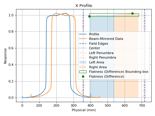
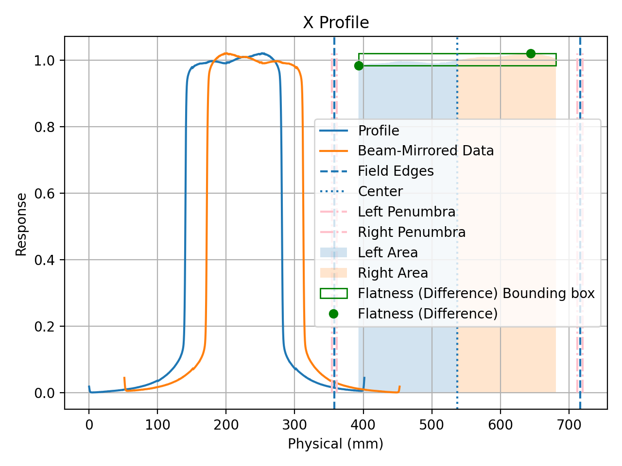
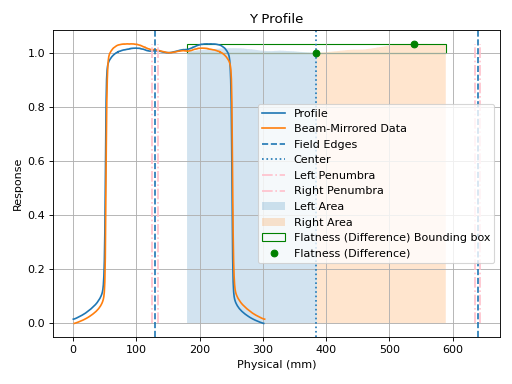
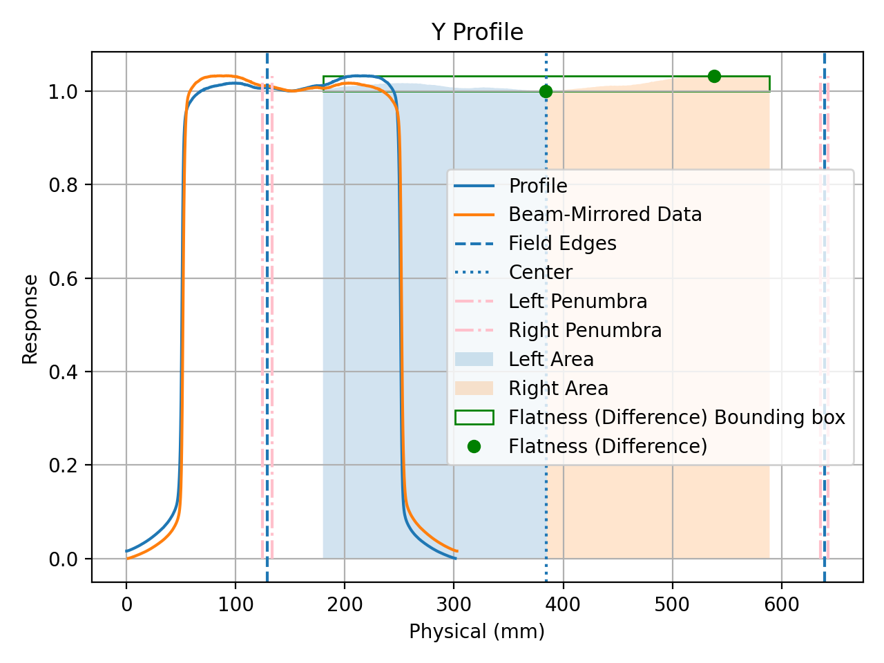
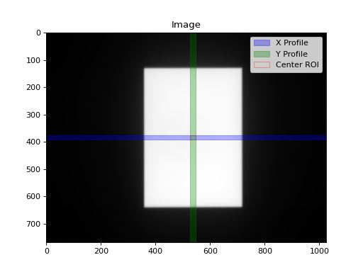
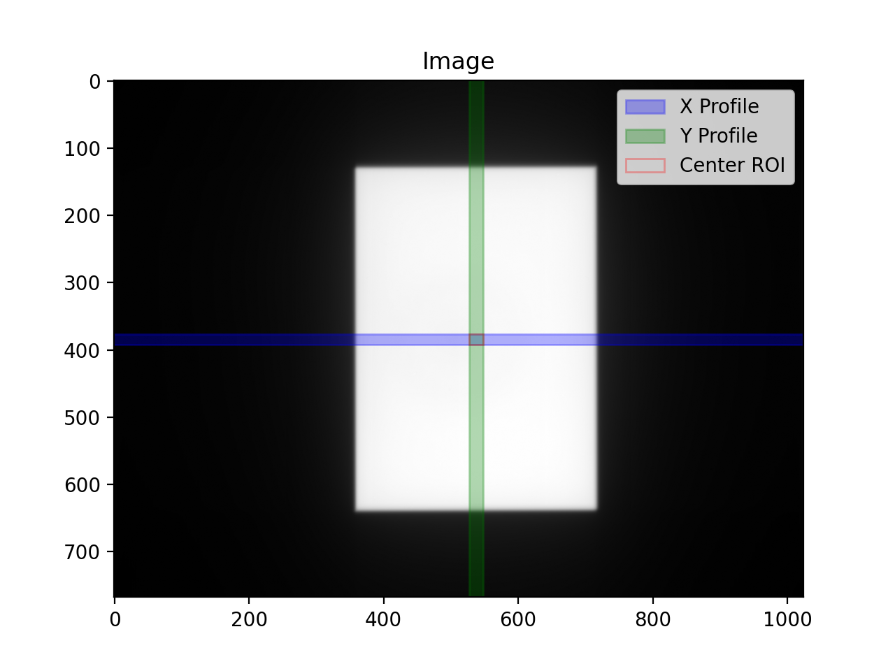
field_analyzer.plot_analyzed_images(show_grid=True, mirror="beam")

which will output 3 images: the image itself marked with where the profiles were taken and the X and Y profile plots along with the metrics plotted.

(Source code)

(png, hires.png, pdf)¶

Analysis Options¶

Centering¶

There are 3 centering options: manual, beam center, and geometric center.

Manual¶

Manual centering means that you as the user specify the position of the image that the profiles are taken from.

from pylinac import FieldProfileAnalysis, Centering

fa = FieldProfileAnalysis(...)
fa.analyze(..., centering=Centering.MANUAL)  # default is the middle of the image.

# or specify a custom location
fa.analyze(..., centering=Centering.MANUAL, position=(0.3, 0.8))
# take profile at 30% height and 80% width

Beam center¶

This is the default centering option. It first looks for the field to find the approximate center along each axis. Then it extracts the profiles at these coordinates. This is helpful if you always want to be near the center of the field, even for offset fields or wedges.

from pylinac import FieldProfileAnalysis, Centering

fa = FieldProfileAnalysis(...)
fa.analyze(...)  # nothing special needed as it's the default

# Specifying a position here will be ignored
fa.analyze(..., centering=Centering.BEAM_CENTER, position=(0.1, 0.4))
# this is allowed but will result in the same result as above

Geometric center¶

The geometric center will always find the middle pixel and extract the profiles from there. This is helpful if you always want to be at the center of the image.

from pylinac import FieldProfileAnalysis, Centering

fa = FieldProfileAnalysis(...)
fa.analyze(..., centering=Centering.GEOMETRIC_CENTER)

Edge detection¶

Edge detection is important for determining the field width and beam center (which is often used for symmetry). There are 3 detection strategies: FWHM, inflection via derivative, and inflection via the Hill/sigmoid/4PNLR function.

FWHM¶

The full-width half-max strategy is traditional and works for flat beams. It can give poor values for FFF beams.

from pylinac import FieldProfileAnalysis, Edge

fa = FieldProfileAnalysis(...)
fa.analyze(..., edge_type=Edge.FWHM)

Inflection (derivative)¶

The inflection point via the derivative is useful for both flat and FFF beams, and is thus the default for FieldProfileAnalysis. The method will find the positions of the max and min derivative of the values. Using a 0-crossing of the 2nd derivative can be tripped up by noise so it is not used.

Note

This method is recommended for high spatial resolution images such as the EPID, where the derivative has several points to use at the beam edge. It is not recommended for 2D device arrays.

from pylinac import FieldProfileAnalysis, Edge

fa = FieldProfileAnalysis(...)  # nothing special needed as it's the default

# you may also specify the edge smoothing value. This is a gaussian filter applied to the derivative just for the purposes of finding the min/max derivative.
# This is to ensure the derivative is not caught by some noise. It is usually not necessary to change this.
fa = FieldProfileAnalysis(..., edge_smoothing_ratio=0.005)

Inflection (Hill)¶

The inflection point via the Hill function is useful for both flat and FFF beams The fitting of the function is best for low-resolution data. The Hill function, the sigmoid function, and 4-point non-linear regression belong to a family of logistic equations to fit a dual-curved value. Since these fit a function to the data the resolution problems are eliminated. Some examples can be seen here. The generalized logistic function has helpful visuals as well here.

The function used here is:

\(f(x) = A + \frac{B - A}{1 + \frac{C}{x}^D}\)

where \(A\) is the low asymptote value (~0 on the left edge of a field), \(B\) is the high asymptote value (~1 for a normalized beam on the left edge), \(C\) is the inflection point of the sigmoid curve, and \(D\) is the slope of the sigmoid.

The function is fitted to the edge data of the field on each side to return the function. From there, the inflection point, penumbra, and slope can be found.

Note

This method is recommended for low spatial resolution images such as 2D device arrays, where there is very little data at the beam edges. While it can be used for EPID images as well, the fit can have small errors as compared to the direct data. The fit, however, is much better than a linear or even spline interpolation at low resolutions.

from pylinac import FieldProfileAnalysis, Edge

fa = FieldProfileAnalysis(..., edge_type=Edge.INFLECTION_HILL)

# you may also specify the Hill window. This is the size of the window (as a ratio) to use to fit the field edge to the Hill function.
fa = FieldProfileAnalysis(..., edge_type=Edge.INFLECTION_HILL, hill_window_ratio=0.05)
# i.e. use a 5% field width about the edges to fit the Hill function.

Note

When using this method, the fitted Hill function will also be plotted on the image. Further, the exact field edge marker (green x) may not align with the Hill function fit. This is just a rounding issue due to the plotting mechanism. The field edge is really using the Hill fit under the hood.

Normalization¶

There are 4 options for interpolation: NONE, GEOMETRIC_CENTER, BEAM_CENTER, and MAX. These should be self-explanatory, especially in light of the centering explanations.

from pylinac import FieldProfileAnalysis, Normalization

fa = FieldProfileAnalysis(...)
fa.analyze(..., normalization_method=Normalization.BEAM_CENTER)

Choosing Metrics¶

The metrics the user can use in the field/profile analysis that come out of the box can be viewed in this list: Built-in Plugins. These metrics can then be passed to the metrics parameter. The user can mix and match as desired. It’s also possible to write custom plugins; see Using Custom Plugins.

from pylinac import FieldProfileAnalysis
from pylinac.metrics.profile import PenumbraRightMetric, SlopeMetric, SymmetryAreaMetric

p = Path(r"C:\path\to\open_field.dcm")
field_analyzer = FieldProfileAnalysis(p)
field_analyzer.analyze(
    metrics=[PenumbraRightMetric(), SlopeMetric(), SymmetryAreaMetric()]
)
field_analyzer.plot_analyzed_images()

Customizing Metrics¶

To change the name or parameters of a metric, pass the relevant parameters to the metric’s constructor. E.g. to use 90/10 for the penumbra distance instead of 80/20:

from pylinac import FieldProfileAnalysis
from pylinac.metrics.profile import PenumbraRightMetric

fa = FieldProfileAnalysis(...)
fa.analyze(metrics=[PenumbraRightMetric(lower=10, upper=90, color="r", ls="--")])
# will use 90/10 instead of 80/20 and plot the line in red and dashed
fa.plot_analyzed_images()

Each metric has its own parameters that can be customized. See the metric’s documentation for more information.

Interpreting results¶

Results from the analysis can be printed as a simple string using results(). The ideal method is to access the results using the results_data() method, which can return a JSON string, a dictionary, or a FieldResult that can be used to access the results.

Using Custom Plugins¶

To analyze custom metrics on the profiles, the user can write custom plugins. First, create the plugin itself. Then, pass it to the metrics parameter per Choosing Metrics.

from pylinac import FieldProfileAnalysis
from pylinac.metrics.profile import PenumbraLeftMetric
from my_custom_plugins import MyCustomMetric

p = Path(r"C:\path\to\open_field.dcm")
field_analyzer = FieldProfileAnalysis(p)
field_analyzer.analyze(metrics=[MyCustomMetric(), PenumbraLeftMetric()])
field_analyzer.plot_analyzed_images()

Comparison to field analysis v1¶

In comparison to the original Field Analysis module, this updated module:

Almost every metric will result in the same value. E.g. flatness, symmetry, etc. The only times that metrics showed differences was if interpolation was “None”. In such a case, the v1 penumbra may be slightly larger. This is due to the field edge index “snapping” to the nearest pixel. In v2, the edge is always interpolated and never snaps.
Is much easier and more logical to write new plugins for. The plugins are modular and are not tightly coupled to this module.
Is loosely coupled to the metrics themselves. Since the metrics themselves are self-contained, can be customized directly, and don’t rely on any specific data massaging or formatting, they can be used in other modules.
Does not do any device-specific analysis (e.g. IC Profiler). The original module and intent was to have a generic device-to-profile framework. This ended up being a considerable amount of work and ultimately we felt it fell out of the scope of pylinac, which is to focus on image analysis. If you desire device-specific profile analysis, the conversion from the original file/format a 1D array of values is your responsibility.
There is no explicit interpolation method. Values are always interpolated linearly under the hood.
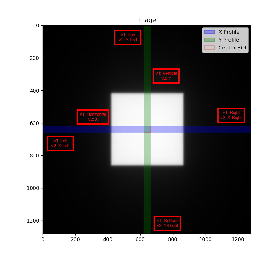
v1 uses language like “top, left, bottom, right”. In v2 everything is left and right, including the y-profile (vertical). Rotating the y-profile 90 degrees counterclockwise will give the same understanding of language. I.e. the “top” is the y-left value.
While not strictly a user benefit, the modularity of the metrics and the analysis itself makes the codebase much cleaner and easier to maintain (v1 is ~1500 LOC vs v2 at ~400).

API Documentation¶

class pylinac.field_profile_analysis.FieldProfileAnalysis(path: str | Path, **kwargs)[source]¶

Bases: ResultsDataMixin[FieldProfileResult]

Field analysis of a radiation field via profiles.

Parameters¶

path: The path to the image to analyze.
kwargs: Keyword arguments to pass to the image loader.

classmethod from_demo_image()[source]¶: Load the demo image into an instance.

analyze(centering: Centering = Centering.BEAM_CENTER, position: tuple[float, float]=(0.5, 0.5), x_width: float | int = 0.0, y_width: float | int = 0.0, normalization: Normalization = Normalization.NONE, edge_type: Edge = Edge.INFLECTION_DERIVATIVE, invert: bool = False, ground: bool = True, metrics: Sequence[ProfileMetric] = (<pylinac.metrics.profile.FlatnessDifferenceMetric object>, <pylinac.metrics.profile.SymmetryPointDifferenceMetric object>, <pylinac.metrics.profile.PenumbraRightMetric object>, <pylinac.metrics.profile.PenumbraLeftMetric object>, <pylinac.metrics.profile.CAXToLeftEdgeMetric object>, <pylinac.metrics.profile.CAXToRightEdgeMetric object>), **kwargs)[source]¶

Analyze the field by pulling out profiles at the specified position and width. The profiles are then analyzed for the given metrics.

Parameters¶

centering: The centering method to use.
position: The relative position of the field to pull the profile in (height, width). E.g. (0.3, 0.6) will pull profiles at 30% of the image height (from the top) and 60% of the image width (from the left).

Note

This is only used if centering is set to ‘manual’.
x_width: The x-width ratio of the field to extract into the profile. Must be between 0 and 1. The pixels are averaged along the width to create the profile.
y_width: The y-width ratio of the field to extract into the profile. Must be between 0 and 1. The pixels are averaged along the height to create the profile.
normalization: The normalization method to use.
edge_type: The type of profile to use. Options are ‘FWXM’, ‘Hill’, and ‘Inflection’.
invert: Whether to invert the image before analyzing.
ground: Whether to “ground” the profile by subtracting the minimum value from all values.
metrics: The metrics to compute on the profiles. Should be a sequence of individual metrics.

results() → str[source]¶: Return a string representation of the results.

plot_analyzed_images(show: bool = True, show_field_edges: bool = True, show_center: bool = True, show_grid: bool = True, mirror: Literal['beam', 'geometry'] | None = None, **kwargs) → list[Figure][source]¶

Plot the analyzed image and x and y profiles.

Parameters¶

show: Whether to show the plots.
show_field_edges: Whether to show the edges of the field of the profiles as vertical lines.
show_center: Whether to show the center of the field as a vertical line on the profiles.
show_grid: Whether to display a grid for the profiles.
mirror: Whether to mirror the image. Options are ‘beam’, ‘geometry’, or None.
kwargs: Additional keyword arguments to pass to the plt.subplots() method.

Returns¶

list[plt.Figure]: The figures of the x profile, y profile, and image.

publish_pdf(filename: str, notes: str | list[str] = None, open_file: bool = False, metadata: dict = None, logo: Path | str | None = None, plot_kwargs: dict | None = None) → None[source]¶

Publish (print) a PDF containing the analysis, images, and quantitative results.

Parameters¶

filename(str, file-like object}: The file to write the results to.
notesstr, list of strings: Text; if str, prints single line. If list of strings, each list item is printed on its own line.
open_filebool: Whether to open the file using the default program after creation.
metadatadict: Extra stream to be passed and shown in the PDF. The key and value will be shown with a colon. E.g. passing {‘Author’: ‘James’, ‘Unit’: ‘TrueBeam’} would result in text in the PDF like: ————– Author: James Unit: TrueBeam ————–
logo: Path, str: A custom logo to use in the PDF report. If nothing is passed, the default pylinac logo is used.
plot_kwargsdict: Additional keyword arguments to pass to the plot_analyzed_image method. E.g. show_grid=False.

clear_captured_warnings() → None¶: Clear the list of captured warnings.

get_captured_warnings() → list[dict]¶: Retrieve the list of captured warnings, deduplicated.

results_data(as_dict: bool = False, as_json: bool = False, by_alias: bool = False, exclude: set[str] | None = None) → T | dict | str¶

Present the results data and metadata as a dataclass, dict, or tuple. The default return type is a dataclass.

Parameters¶

as_dictbool: If True, return the results as a dictionary.
as_jsonbool: If True, return the results as a JSON string. Cannot be True if as_dict is True.
by_aliasbool: If True, use the alias names of the dataclass fields. These are generally the more human-readable names.
excludeset: A set of fields to exclude from the results data.

pydantic model pylinac.field_profile_analysis.FieldProfileResult[source]¶

Bases: ResultBase

Create a new model by parsing and validating input data from keyword arguments.

Raises [ValidationError][pydantic_core.ValidationError] if the input data cannot be validated to form a valid model.

self is explicitly positional-only to allow self as a field name.

field x_metrics: dict [Required]¶

The metrics computed from the X/crossplane profile. The items included depend on the metrics given to the analysis. See: Built-in Plugins. The key will be the name of the metric and the value will be what’s returned from the calculate method of the metric. In addition, the following items are always given:

Field Width (mm): The width of the field in mm.
values: A list of pixel values of the profile that the metrics were calculated from.

field y_metrics: dict [Required]¶

Field Width (mm): The width of the field in mm.
values: A list of pixel values of the profile that the metrics were calculated from.

field center: dict [Required]¶: The center ROI of the field

field normalization: str [Required]¶: The normalization method used.

field edge_type: str [Required]¶: The edge detection method used.

field centering: str [Required]¶: The centering method used.