Winston-Lutz¶

Overview¶

The Winston-Lutz module loads and processes EPID images that have acquired Winston-Lutz type images.

Features:

Couch shift instructions - After running a WL test, get immediate feedback on how to shift the couch. Couch values can also be passed in and the new couch values will be presented so you don’t have to do that pesky conversion. “Do I subtract that number or add it?”
Automatic field & BB positioning - When an image or directory is loaded, the field CAX and the BB are automatically found, along with the vector and scalar distance between them.
Isocenter size determination - Using backprojections of the EPID images, the 3D gantry isocenter size and position can be determined independent of the BB position. Additionally, the 2D planar isocenter size of the collimator and couch can also be determined.
Image plotting - WL images can be plotted separately or together, each of which shows the field CAX, BB and scalar distance from BB to CAX.
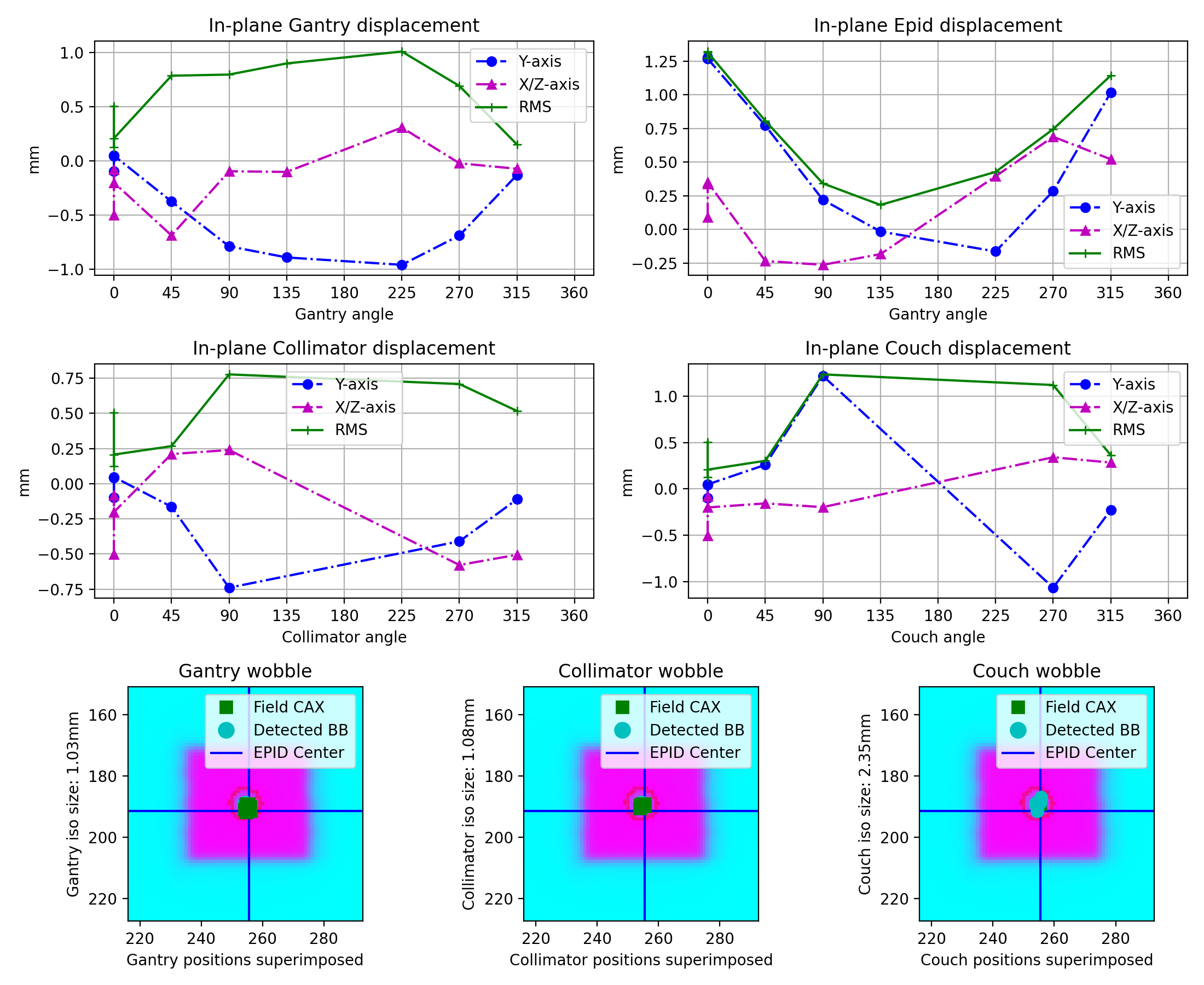
Axis deviation plots - Plot the variation of the gantry, collimator, couch, and EPID in each plane as well as RMS variation.
File name interpretation - Rename DICOM filenames to include axis information for linacs that don’t include such information in the DICOM tags. E.g. “myWL_gantry45_coll0_couch315.dcm”.

Warning

Documentation often uses the term “field CAX” or “CAX” to refer to the center of the radiation field. This is something of a misnomer and we apologize in advance. Due to backwards-compatibility reasons, the term continues to be used in the code and documentation.

Running the Demo¶

To run the Winston-Lutz demo, create a script or start an interpreter session and input:

from pylinac import WinstonLutz

WinstonLutz.run_demo()

Results will be printed to the console and a figure showing the zoomed-in images will be generated:

Winston-Lutz Analysis
=================================
Number of images: 17
Maximum 2D CAX->BB distance: 1.23mm
Median 2D CAX->BB distance: 0.69mm
Shift to iso: facing gantry, move BB: RIGHT 0.36mm; OUT 0.36mm; DOWN 0.20mm
Gantry 3D isocenter diameter: 1.05mm (9/17 images considered)
Maximum Gantry RMS deviation (mm): 1.03mm
Maximum EPID RMS deviation (mm): 1.31mm
Gantry+Collimator 3D isocenter diameter: 1.11mm (13/17 images considered)
Collimator 2D isocenter diameter: 1.09mm (7/17 images considered)
Maximum Collimator RMS deviation (mm): 0.79
Couch 2D isocenter diameter: 2.32mm (7/17 images considered)
Maximum Couch RMS deviation (mm): 1.23

(Source code, png, hires.png, pdf)

Image Acquisition¶

The Winston-Lutz module will only load EPID images. The images can be from any EPID however, and any SID. To ensure the most accurate results, a few simple tips should be followed. Note that these are not unique to pylinac; most Winston-Lutz analyses require these steps:

The BB should be fully within the field of view.
The MLC field should be symmetric.

Prefabricated plans are available at Pre-Generated Plans for download. See also the Plan Generator module for creating your own plans.

Axis Values¶

Pylinac uses the Image types & output definitions definition to bin images. Regardless of the axis values, pylinac will calculate some values like max/median BB->CAX distance. Other values such as gantry iso size will only use Reference and Gantry image types as defined in the linked section. We recommend reviewing the analysis definitions and acquiring images according to the values you are interested in. Some examples are below. Note that these are not mutually exclusive:

Simple max distance to BB: Any axis values; any combination of axis values are allowed.
Gantry iso size: Gantry value can be any; all other axes must be 0.
Collimator iso size: Collimator value can be any; all other axes must be 0.

If, e.g., all axis values are combinations of axes then gantry iso size will not be calculated. Further, the plot_analyzed_image method assumes Gantry, Collimator, and/or Couch image sets. If only combinations are passed, this image will be empty. A good practice is also to acquire a reference image if possible, meaning all axes at 0.

Coordinate Space¶

Note

In pylinac 2.3, the coordinates changed to be compliant with IEC 61217. Compared to previous versions, the Y and Z axis have been swapped. The new Z axis has also flipped which way is positive.

When interpreting results from a Winston-Lutz test, it’s important to know the coordinates, origin, etc. Pylinac uses IEC 61217 (FIXED) coordinate space for Cartesian shifts. Colloquial descriptions are as if standing at the foot of the couch looking at the gantry.

X-axis - Lateral, or left-right, with right being positive.
Y-axis - Superior-Inferior, or in-out, with sup/in being positive.
Z-axis - Anterior-Posterior, or up-down, with up/anterior being positive.

Passing a coordinate system¶

Added in version 3.6.

Warning

If using DICOM images that include the gantry (300A,011E), collimator (300A,0120), and couch (300A,0122) tags, they will be in IEC61217, regardless of what coordinate system is set up locally. I.e. if you use Varian IEC, the machine values locally will follow this convention, but when saved to DICOM, they will be converted to IEC61217 under the hood for you.

You should only need to change the coordinate system when also using the axis_mapping parameter in analyze.

It is possible to pass in your machine’s coordinate scale/system to the analyze parameter like so:

from pylinac.winston_lutz import WinstonLutz, MachineScale

wl = WinstonLutz(...)
wl.analyze(..., machine_scale=MachineScale.VARIAN_IEC)
...

This will change the BB shift vector and shift instructions accordingly. If you don’t use the shift vector or instructions then you won’t need to worry about this parameter.

Typical Use¶

Analyzing a Winston-Lutz test is simple. First, let’s import the class:

from pylinac import WinstonLutz

From here, you can load a directory:

my_directory = "path/to/wl_images"
wl = WinstonLutz(my_directory)

You can also load a ZIP archive with the images in it:

wl = WinstonLutz.from_zip("path/to/wl.zip")

Now, analyze it:

wl.analyze(bb_size_mm=5)

And that’s it! You can now view images, print the results, or publish a PDF report:

# plot all the images
wl.plot_images()
# plot an individual image
wl.images[3].plot()
# save a figure of the image plots
wl.save_plots("wltest.png")
# print to PDF
wl.publish_pdf("mywl.pdf")

If you want to shift the BB based on the results and perform the test again there is a method for that:

print(wl.bb_shift_instructions())
# LEFT: 0.1mm, DOWN: 0.22mm, ...

You can also pass in your couch coordinates and the new values will be generated:

print(wl.bb_shift_instructions(couch_vrt=0.41, couch_lng=96.23, couch_lat=0.12))
# New couch coordinates (mm): VRT: 0.32; LNG: 96.11; LAT: 0.11

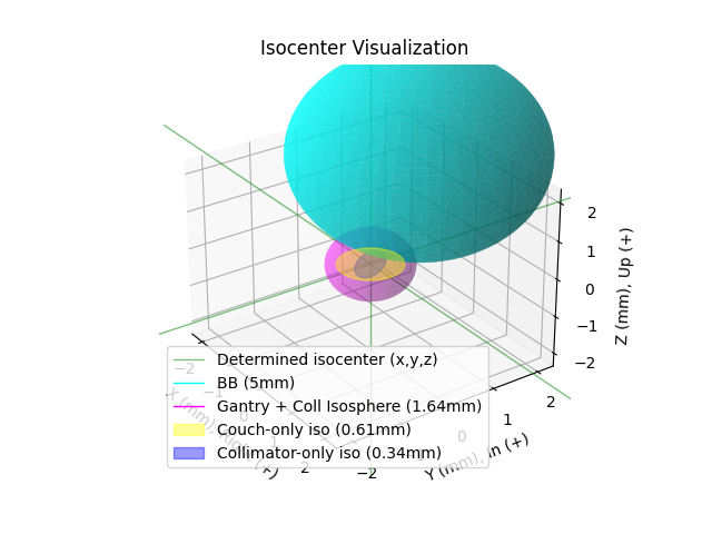
Visualizing the Isocenter-to-BB¶

Added in version 3.17.

The isocenter and BB can be visualized together after analysis by calling plot_location:

wl = WinstonLutz(...)
wl.analyze(...)
wl.plot_location()

This will result in a 3D plot visualizing the BB (true physical size) and the isocenter (true physical size) in the room coordinates like so:

Accessing data¶

Changed in version 3.0.

Using the WL module in your own scripts? While the analysis results can be printed out, if you intend on using them elsewhere (e.g. in an API), they can be accessed the easiest by using the results_data() method which returns a WinstonLutzResult instance.

Note

While the pylinac tooling may change under the hood, this object should remain largely the same and/or expand. Thus, using this is more stable than accessing attrs directly.

Continuing from above:

data = wl.results_data()
data.num_total_images
data.max_2d_cax_to_bb_mm
# and more

# return as a dict
data_dict = wl.results_data(as_dict=True)
data_dict["num_total_images"]
...

Accessing individual images¶

Each image can be plotted and otherwise accessed easily:

wl = WinstonLutz(...)
# access first image
wl.images[
    0
]  # these are subclasses of the pylinac.core.image.DicomImage class, with a few special props
# plot 3rd image
wl.images[
    0
].plot()  # the plot method is special to the WL module and shows the BB, EPID, and Field CAX.
# get 2D x/y vector of an image
wl.images[
    4
].cax2bb_vector  # this is a Vector with a .x and .y attribute. Note that x and y are in respect to the image, not the fixed room coordinates.

Analyzing a single image¶

You may optionally analyze a single image if that is your preference. Obviously, no 3D computations are performed.

Note

This is the same class used under the hood for the WinstonLutz images, so any attribute you currently use with something like wl.images[2].cax2bb_vector will work for the below with a direct call: wl2d.cax2bb_vector.

from pylinac import WinstonLutz2D

wl2d = WinstonLutz2D("my/path/...")
wl2d.analyze(bb_size_mm=4)  # same as WinstonLutz class
wl2d.plot()
...

This class does not have all the methods that WinstonLutz has for mostly obvious reasons and lower likelihood of being used directly.

Passing in Axis values¶

Important

When passing in axis values manually, you can also use machine_scale in conjunction to specify the coordinate system you are stating the axes to be in. See Passing a coordinate system.

If your linac EPID images do not include axis information (such as Elekta) there are two ways to pass the data in.

via filenames¶

First, you can specify it in the file name. Any and all of the three axes can be defined. If one is not defined and is not in the DICOM tags, it will default to 0. The syntax to define the axes: “<*>gantry0<*>coll0<*>couch0<*>”. There can be any text before, after, or in between each axis definition. However, the axes numerical value must immediately follow the axis name. Axis names are also fixed. The following examples are valid:

MyWL-gantry0-coll90-couch315.dcm
gantry90_stuff_coll45-couch0.dcm
abc-couch45-gantry315-coll0.dcm
01-gantry0-abcd-coll30couch10abc.dcm
abc-gantry30.dcm
coll45abc.dcm

The following are invalid:

mywl-gantry=0-coll=90-couch=315.dcm
gan45_collimator30-table270.dcm

Using the filenames within the code is done by passing the use_filenames=True flag to the init method:

my_directory = "path/to/wl_images"
wl = WinstonLutz(my_directory, use_filenames=True)

Note

If using filenames any relevant axes must be defined, otherwise they will default to zero. For example, if the acquisition was at gantry=45, coll=15, couch=0 then the filename must include both the gantry and collimator in the name (<…gantry45…coll15….dcm>). For this example, the couch need not be defined since it is 0.

via `axis_mapping`¶

The other way of inputting axis information is passing the axis_mapping parameter to the constructor. This is a dictionary with the filenames as keys and a tuple of ints for the gantry, coll, and couch:

directory = "path/to/wl/dir"
mapping = {
    "file1.dcm": (0, 0, 0),
    "file2.dcm": (90, 315, 45),
}  # add more as needed
wl = WinstonLutz(directory=directory, axis_mapping=mapping)
# analyze as normal
wl.analyze(...)

Note

The filenames should be local to the directory. In the above example the full paths would be path/to/wl/dir/file1.dcm, and path/to/wl/dir/file2.dcm.

Setting Reference Axis Values¶

It is possible to set reference axis values to angles other than zero. E.g. if the intended collimator angle of reference is 45 degrees to average the collimator rotation of a VMAT plan. In addition to changing reference values, the “snap” tolerance can also be passed which will allow axis angles to “snap” if the axis value is within the snap tolerance. See Image types & output definitions. This can be helpful for scenarios where you forgot to set the couch axes to 0 from a previous CBCT shift.

To change the reference values and set a snap tolerance of 5 degrees:

wl = WinstonLutz(...)
wl.analyze(
    ...,
    snap_tolerance=5,
    gantry_reference=45,
    collimator_reference=10,
    couch_reference=0,
)

In the above scenario, images with gantry ranges of 40-50 degrees, collimator 5-15, and couch 355-5 will be considered “Reference” images.

This can also be helpful if you have a very old linac and or use a coordinate space such as Varian Standard where gantry 180 is pointing to the floor, in which case you can set the gantry reference to 180.

Note

The snap tolerance does not actually change the axis values, just the variable Axis type.

Changing BB detection size¶

To change the size of BB pylinac is expecting you can pass the size to the analyze method:

import pylinac

wl = WinstonLutz(...)
wl.analyze(bb_size_mm=3)
...

Low-density BBs¶

If using a phantom with a BB that has a lower density that than the surrounding material, pass the low_density_bb parameter:

import pylinac

wl = WinstonLutz(...)
wl.analyze(..., low_density_bb=True)
...

kV Analysis/Imaging-only iso evaluation¶

It is possible to analyze kV WL images and/or analyze a WL set and only focus on the imaging iso. In this case there are two parameters you likely need to adjust: open_field and low_density_bb. The first will set the field center to the image center. It is assumed the field is not of interest or the field cannot be measured, such as a fully-open kV image. Use this anytime the radiation iso is not of interest. For large-field WL images, you may need to set the low_density_bb parameter to True. This is because the automatic inversion of the WL module assumes a small field is being delivered. For large field deliveries, kV or MV, see about flipping this parameter if the analysis fails.

CBCT Analysis¶

Added in version 3.16.

Warning

This feature is still experimental. Use with caution.

It’s possible to take and load a CBCT dataset of a BB using the from_cbct and from_cbct_zip class methods. The CBCT dataset is loaded as a 3D numpy array. Projections at the 4 faces of the array (top, left, bottom, right) are created into pseudo-cardinal angle DICOMs. These DICOMs are then loaded as normal images and analyzed.

Example of loading and analyzing a CBCT dataset of a WL BB¶

wl = WinstonLutz.from_cbct("my/cbct/dir")
# OR
wl = WinstonLutz.from_cbct_zip("my/cbct.zip")
# ensure to set low density and open field to True
wl.analyze(low_density_bb=True, open_field=True, bb_size_mm=3)
# use as normal
print(wl.results())
print(wl.results_data())
print(wl.bb_shift_instructions())
wl.plot_images()

Warning

The CBCT analysis comes with a few caveats:

Analyzing the image will override the low_density_bb and open_field flags to always be True; it does not matter what is passed in analyze.
No axis deviation information is available, i.e. couch/coll/gantry walkout.
There are always 4 images generated.
The generated images are not true DICOMs and thus do not have all the DICOM tags.

Virtual Shifting¶

Added in version 3.22.

It is possible to virtually shift the BB for regular WL images to see what the 2D errors of the images would be if the BB were shifted to the optimal position. This can help avoid iterating on the nominal BB position by physically moving the BB.

To virtually move the BB, pass apply_virtual_shift to the analyze method:

wl = WinstonLutz(...)
wl.analyze(..., apply_virtual_shift=True)
...

This will result in images where the detected BB plotted does not overlap with the apparent BB location for obvious reasons.

The results will be the same as if the BB were physically moved to the optimal position. The results will be slightly different and report what the virtual shift was. This is simply the original BB shift instructions before the shift.

Note

This only affects the 2D error results. One of the benefits of pylinac is that the iso size for gantry, couch, and collimator are done independent of the BB position.

Using TIFF images¶

Added in version 3.12.

The WL module can handle TIFF images on a provisional basis.

Warning

This is still experimental and caution is warranted. Even though there is an automatic noise/edge cleaner, cropping images to remove markers and/or film scan artifacts is encouraged.

To load TIFF images, extra parameters must be passed. Specifically, the sid and potentially the dpi parameters must be added. Additionally, axis_mapping must be populated. This is how pylinac can convert the images into rudimentary dicom images. The dpi parameter is only needed if the TIFF images do not have a resolution tag. Pylinac will give a specific error if dpi wasn’t passed and also wasn’t in the TIFF tags.

Note

Although it is technically possible to load both DICOM and TIFF together in one dataset it is not encouraged.

from pylinac import WinstonLutz

my_tiff_images = list(Path(...), Path(...))
wl_tiff = WinstonLutz(
    my_tiff_images,
    sid=1000,
    dpi=212,
    axis_mapping={"g0.tiff": (0, 0, 0), "g270.tiff": (270, 0, 0)},
)
# now analyze as normal
wl_tiff.analyze(...)
print(wl_tiff.results())

Note that other .from... methods are available such as .from_zip:

from pylinac import WinstonLutz

my_tiff_zip = "../files/tiffs.zip"
# same inputs as above
wl_tiff = WinstonLutz.from_zip(my_tiff_zip, dpi=...)

Image types & output definitions¶

The following terms are used in pylinac’s WL module and are worth defining.

Image axis definitions/Image types Images are classified into 1 of 6 image types, depending on the position of the axes. The image type is then used for determining whether to use the image for the given calculation. Image types allow the module to isolate the analysis to a given axis if needed. E.g. for gantry iso size, as opposed to overall iso size, only the gantry should be moving so that no other variables influence it’s calculation.

Note

Reference value defaults are 0, but this can be changed. See Setting Reference Axis Values.

Reference: This is when all axes are at the reference value (default 0; e.g. gantry=coll=couch=0).
Gantry: This is when all axes but gantry are at the reference value; e.g. gantry=45, coll=0, couch=0.
Collimator: This is when all axes but collimator are at the reference value.
Couch: This is when all axes but the couch are at the reference value.
GB Combo: This is when either the gantry or collimator are non-zero but the couch is at the reference value.
GBP Combo: This is where the couch is kicked and the gantry and/or collimator are rotated away from reference.

Analysis definitions Given the above terms, the following calculations are performed.

Maximum 2D CAX->BB distance (scalar, mm): Analyzes all images individually for the maximum 2D distance from rad field center to the BB.
Median 2D CAX->BB distance (scalar, mm): Same as above but the median.
Shift of BB to isocenter (vector, mm): The instructions of how to move the BB/couch in order to place the BB at the determined isocenter.
Gantry 3D isocenter diameter (scalar, mm): Analyzes only the gantry axis images (see above image types). Applies backprojection of the CAX in 3D and then minimizes a sphere that touches all the 3D backprojection lines.
Gantry+Collimator 3D isocenter diameter (scalar, mm): Same as above but also considers Collimator and GB Combo images.
[Couch, Collimator] 2D isocenter diameter (scalar, mm): Analyzes only the collimator or couch images to determine the size of the isocenter according to the axis in question. The maximum distance between any of the points is the isocenter size. The couch and collimator are treated separately for obvious reasons. If no images are given that rotate about the axis in question (e.g. cardinal gantry angles only) the isocenter size will default to 0.
[Maximum, All][Gantry, Collimator, Couch, GB Combo, GBP Combo, EPID] RMS deviation (array of scalars, mm): Analyzes the images for the axis in question to determine the overall RMS inclusive of all 3 coordinate axes (vert, long, lat). I.e. this is the overall displacement as a function of the axis in question. For EPID, the displacement is calculated as the distance from image center to BB for all images with couch=0. If no images are given that rotate about the axis in question (e.g. cardinal gantry angles only) the isocenter size will default to 0.

Interpreting Results¶

This explains the WinstonLutzResult class that is returned from the results_data method. This is also what is given in RadMachine image analysis results and is explained further here.

num_gantry_images: The number of images that were taken at different gantry angles and all other axes were at reference.
num_gantry_coll_images: The number of images that were taken at different gantry and collimator angles and the couch was at reference.
num_coll_images: The number of images that were taken at different collimator angles and all other axes were at reference.
num_couch_images: The number of images that were taken at different couch angles and all other axes were at reference.
num_total_images: The total number of images analyzed.
max_2d_cax_to_bb_mm: The maximum 2D distance from the field CAX to the BB across all images analyzed in mm.
median_2d_cax_to_bb_mm: The median 2D distance from the field CAX to the BB across all images analyzed in mm.
mean_2d_cax_to_bb_mm: The mean 2D distance from the field CAX to the BB across all images analyzed in mm.
max_2d_cax_to_epid_mm: The maximum 2D distance from the field CAX to the EPID center across all images analyzed in mm.
median_2d_cax_to_epid_mm: The median 2D distance from the field CAX to the EPID center across all images analyzed in mm.
mean_2d_cax_to_epid_mm: The mean 2D distance from the field CAX to the EPID center across all images analyzed in mm.
gantry_3d_iso_diameter_mm: The 3D isocenter diameter of the gantry axis only as determined by the gantry images in mm. This uses backprojection lines of the field center to the source and minimizes a sphere that touches all the backprojection lines.

Note

This value is independent of the BB position.
max_gantry_rms_deviation_mm: The maximum RMS value of the field CAX to BB for the gantry axis images in mm. This is an alternative to the max/mean/median calculations.
max_epid_rms_deviation_mm: The maximum RMS value of the field CAX to EPID center for the EPID images in mm. This is an alternative to the max/mean/median calculations.
gantry_coll_3d_iso_diameter_mm: The 3D isocenter diameter of the gantry and collimator axes as determined by the gantry and collimator images in mm.
coll_2d_iso_diameter_mm: The 2D isocenter diameter of the collimator axis only as determined by the collimator images in mm.
max_coll_rms_deviation_mm: The maximum RMS deviation of the field CAX to BB for the collimator axis images in mm. This is an alternative to the max/mean/median calculations.
max_couch_rms_deviation_mm: The maximum RMS value of the field CAX to BB for the couch axis images in mm. This is an alternative to the max/mean/median calculations. This uses backprojection lines of the field center to the source and minimizes a sphere that touches all the backprojection lines.

Note

This value is independent of the BB position.
couch_2d_iso_diameter_mm: The 2D isocenter diameter of the couch axis only as determined by the couch images in mm.
bb_shift_vector: The Cartesian vector that would move the BB to the radiation isocenter. Each value is in mm. See also Virtual Shifting, Couch shift
image_details: A list of the individual image results. Each item has the following:
- variable_axis: The axis that varied in the image. See Image types & output definitions.
- bb_location: The location of the BB in the image as a Point in pixels.
- cax2epid_vector: The vector (in Cartesian coordinates) from the field CAX to the EPID center in mm.
- cax2epid_distance: The distance from the field CAX to the EPID center in mm.
- cax2bb_vector: The vector (in Cartesian coordinates) from the field CAX to the BB in mm.
- cax2bb_distance: The scalar distance from the field CAX to the BB in mm.
- field_cax: The location of the field CAX in the image as a Point in pixels.
keyed_image_details: A dictionary of the individual image results. This is the same as image_details but keyed by the images using the axes values as the key. E.g. G0B45P0. This can be used to identify individual images vs those in image_details.

Interpreting specific publications¶

A common question is how the algorithm is to be matched to existing QA publications. Some publications only specify the test and tolerance and say nothing about implementation. We list the publications and also our interpretation of what they mean. We do not make recommendations about how something should be done, but given the number of questions on the subject we provide this information.

AAPM TG-142 Table III, Mechanical:. “Coincidence of radiation and mechanical isocenter”. We interpret this to mean: 1) set up a BB at what you believe is the mechanical isocenter (e.g. light field, lasers, etc). 2) Perform a typical WL image dataset. 3) The bb_shift_vector is the value of interest as it’s the vector from BB to the overall radiation isocenter.
AAPM TG-198: 2.D.2.5: TG-198 is an implementation guide of TG-142 and gives explicit guidance. We do not recommend using starshots for iso size analysis, but it can be done. The WL procedure describes placing the BB at the mechanical isocenter via the surrogate of the lasers. The displacement from the determined radiation iso from the images to the BB/mechanical isocenter is the value of interest, that is bb_shift_vector.
MPPG 9.a Table I - Monthly: Fortunately, the guidance is very clear here and is the maximum of any planar image from BB to field center. This is the max_2d_cax_to_bb_mm value.
MPPG 9.a Table I - Annual: This one is less clear but we interpret it as the bb_shift_vector. See also Couch shift.
MPPG 8.b Table 5 - M11, Table 8 MLC4: This is very vague and does not provide any details on implementation other than that it should be jaw-based and MLC-based respectively and should involve the gantry, couch, and collimator. However, they do add a footnote to reference MPPG 9.a (above).

Finally, it is worth nothing that physicists often have strong feelings about how WL should be done and interpreted. While we agree that providing the best possible treatment to patients is paramount, there are many ways that this can be improved, beyond just WL. It is one piece of many to provide high-quality care. Spending inordinate amounts of time squabbling over a pixel or two is time poorly spent. Finally, we argue for an empirical approach, which is why the image generator was created. See: Benchmarking the Algorithm

Analysis Parameters¶

pylinac

See analyze() for details.

RadMachine

BB size: The size of the BB in mm.
Use Filenames: Whether to use the filenames to determine the axis values. See Passing in Axis values.
Low-Density BB: Whether the BB is lower density than the surrounding material. E.g. an air pocket vs a tungsten BB.
Omit field determination: If checked, sets the field center to the EPID center under the assumption the field is not the focus of interest or is too wide to be calculated. This is often helpful for kV WL analysis where the blades are wide open and even then the blade edge is of less interest than simply the imaging iso vs the BB.

Note

For kV WL, you will generally need to check this and also check the low-density BB flag.
Coordinate system: The coordinate system of the machine. This is used to determine the shift instructions. See Passing a coordinate system. This should only be changed if the axis values (gantry, collimator, couch) are being changed or entered manually.
Pixels/inch: The resolution of the images in pixels per inch. This is used to convert the pixel distances to mm.

Note

Only needed for TIFF/non-DICOM images and only if the resolution is not in the TIFF tags.
Source-to-image distance: The source-to-image distance in mm.

Note

Only needed for TIFF/non-DICOM images.
Is a CBCT scan?: Whether the images are from a CBCT scan. If checked, will create 4 DRRs at gantry 0, 90, 180, 270.
Apply virtual shift of BB to optimal isocenter: If checked, will virtually shift the BB to the optimal isocenter position and reanalyze the images. See Virtual Shifting.

Algorithm¶

The Winston-Lutz algorithm is based on the works of Winkler et al, Du et al, and Low et al. Winkler found that the collimator and couch iso could be found using a minimum optimization of the field CAX points. They also found that the gantry isocenter could by found by “backprojecting” the field CAX as a line in 3D coordinate space, with the BB being the reference point. This method is used to find the gantry isocenter size.

Couch shift¶

Low et al determined the geometric transformations to apply to 2D planar images to calculate the shift to apply to the BB. This method is used to determine the shift instructions. Specifically, equations 6, 7, and 9.

Note

If doing research, it is very important to note that Low implicitly used the “Varian” coordinate system. This is an old coordinate system and any new Varian linac actually uses IEC 61217. However, because the gantry and couch definitions are different, the matrix definitions are technically incorrect when using IEC 61217. By default, Pylinac assumes the images are in IEC 61217 scale and will internally convert it to varian scale to be able to use Low’s equations. To use a different scale use the machine_scale parameter, shown here Passing a coordinate system. Also see Machine Scale.

As a prologue, we should explain the differences in our coordinate system vs Low’s. In the paper the gantry coordinate system is defined as such:

“Let \((X_{G},Y_{G},Z_{G})\) represent a gantry coordinate system defined as follows: the \(X_{G}\) axis corresponds to the gantry rotation axis, with its positive direction pointing away from the gantry (toward the couch); the \(Z_{G}\) axis coincides with the central axis of the radiation beam, pointing into the collimator, and the \(Y_{G}\) axis is assigned such that \((X_{G},Y_{G},Z_{G})\) forms a right-handed coordinate system.”

Later in equation 2 they defined a couch coordinate system as:

\[ \begin{align}\begin{aligned}X_{c} = VERT\\Y_{c} = LAT\\Z_{c} = -AP\end{aligned}\end{align} \]

but this is inconsistent because AP is the same as VERT in normal conventions. Using the sentence after eqn 2 as a guide: “A couch angle of \(\phi\) degrees corresponds to a signed rotation around the \(Z_{C}\) axis of the couch coordinate system.”

Just from this sentence it would appear \(Z_{C}\) should be VERT. The only way this makes sense is if the couch coordinate system is from a HFS patient perspective; i.e. VERT=>In/Out, LAT=>Left/Right, -AP=>Up/Down. If this is true, everything falls into place.

Finally, it is worth nothing that in the Varian “Standard” coordinate system (the one assumed by Low), couch vertical increases as the couch is lowered. This may explain the negative sign in the Z axis of equation 2, whereas for the IEC 61217 scale, vertical increases as the couch is raised.

We thus can generate the following table for transforming the equations from Low to IEC 61217/pylinac coordinates:

Low Couch coordinates		Low Couch Axes		Low Gantry coordinates		Low Gantry axes		Pylinac Gantry coordinates
Xc	=	VERT	=	Xg	=	LONG	=	-Y (In/Out)
Yc	=	LAT	=	Yg	=	LAT	=	X (Left/Right)
Zc	=	-AP	=	Zg	=	VERT	=	Z (Up/Down)

See Coordinate Space.

We can now address the implementation for the couch shift as follows:

For each image we determine (equation 6a):

\[\begin{split}\textbf{A}(\phi, \theta) = \begin{pmatrix} -\cos(\phi) & -\sin(\phi) & 0 \\ -\cos(\theta)\sin(\phi) & \cos(\theta)\cos(\phi) & -\sin(\theta) \end{pmatrix}\end{split}\]

where \(\theta\) is the gantry angle and \(\phi\) is the couch angle (Remember, these must be in Varian Standard axes values).

The \(\xi\) matrix is then calculated with an altered equation 7:

\[\xi = (y_{1},-x_{1}, ..., y_{i},-x_{i},..., y_{n},-x_{n})^{T}\]

where \(x_{i}\) and \(y_{i}\) are the scalar shifts from the field CAX to the BB for \(n\) images in our coordinate system.

Note

Equation 7 has \((x_{i},y_{i})\) convention, but we use \((y_{i},-x_{i})\). Using Figure 1 as a guide, it says the x-axis is pointing toward the gantry (and points to the right in the figure). Both the x and y axes appear inverted here. In the figure both \(x_{i}\) and \(y_{i}\) values are presumably positive in the example, but are both negative when using the right-hand rule of Low’s gantry coordinate definition (”…with [\(X_{G}\)] positive direction pointing away from the gantry”). Thus \(x_{i}\) becomes \(-x_{i}\) when using Low’s own coordinate convention. Using the above table conversion this becomes \(y_{i}\). A similar conversion is true for the y-axis.

\[ \begin{align}\begin{aligned}+x_{Fig1} = -x_{Low} = y_{Pylinac}\\+y_{Fig1} = -y_{Low} = -x_{Pylinac}\end{aligned}\end{align} \]

From equation 9 we can calculate \(\textbf{B}(\phi_{1},\theta_{1},..., \phi_{n},\theta_{n})\):

\[\begin{split}\textbf{B} = \begin{pmatrix} \textbf{A}(\phi_{1},\theta_{1}) \\ \vdots \\ \textbf{A}(\phi_{i},\theta_{i}) \\ \vdots \\ \textbf{A}(\phi_{n},\theta_{n}) \end{pmatrix}\end{split}\]

using the above definitions.

We can then solve for the shift vector \(\boldsymbol{\Delta}\):

\[\boldsymbol{\Delta} = \textbf{B}(\phi_{1},\theta_{1},..., \phi_{n},\theta_{n}) \cdot \xi\]

Using our conversion table above, \(\boldsymbol{\Delta}\) resolves to:

\[\begin{split}\boldsymbol{\Delta} = \begin{pmatrix} \Delta \text{VERT} \\ \Delta \text{LAT} \\ \Delta \text{-AP} \end{pmatrix}_{Low} = \begin{pmatrix} \Delta \text{-LONG} \\ \Delta \text{LAT} \\ \Delta \text{VERT} \end{pmatrix}_{Pylinac}\end{split}\]

where \((...)_{Low}\) and \((...)_{Pylinac}\) are in their respective coordinate systems.

Implementation¶

The algorithm works like such:

Allowances

The images can be acquired with any EPID (aS500, aS1000, aS1200) at any SID.
The BB does not need to be near the real isocenter to determine isocenter sizes, but does affect the 2D image analysis.

Restrictions

Warning

Analysis can fail or give unreliable results if any Restriction is violated.

The BB must be fully within the field of view.
The BB must be within 2.0cm of the real isocenter.
The images must be acquired with the EPID.

Analysis

Find the field CAX – The spread in pixel values (max - min) is divided by 2, and any pixels above the threshold is associated with the open field. The pixels are converted to black & white and the center of mass of the pixels is assumed to be the field CAX.
Find the BB – The algorithm for finding the BB can be found here: Algorithm.

Note

Strictly speaking, the following aren’t required analyses, but are explained for fullness and clarity.

Backproject the CAX for gantry images – Based on the vector of the BB to the field CAX and the gantry angle, a 3D line projection of the CAX is constructed. The BB is considered at the origin. Only images where the couch was at 0 are used for CAX projection lines.
Determine gantry isocenter size - Using the backprojection lines, an optimization function is run to minimize the maximum distance to any line. The optimized distance is the isocenter radius.
Determine collimator isocenter size - The maximum distance between any two field CAX locations is calculated for all collimator images.
Determine couch isocenter size - Instead of using the BB as the non-moving reference point, which is now moving with the couch, the Reference image (gantry = collimator = couch = 0) CAX location is the reference. The maximum distance between any two BB points is calculated and taken as the isocenter size.

Note

Collimator iso size is always in the plane normal to the gantry, while couch iso size is always in the x-z plane.

Benchmarking the Algorithm¶

With the image generator module we can create test images to test the WL algorithm on known results. This is useful to isolate what is or isn’t working if the algorithm doesn’t work on a given image and when commissioning pylinac. It is common, especially with the WL module, to question the accuracy of the algorithm. Since no linac is perfect and the results are sub-millimeter, discerning what is true error vs algorithmic error can be difficult. The image generator module is a perfect solution since it can remove or reproduce the former error.

See the Image Generator module for more information and specifically the generate_winstonlutz() function.

Perfect Delivery¶

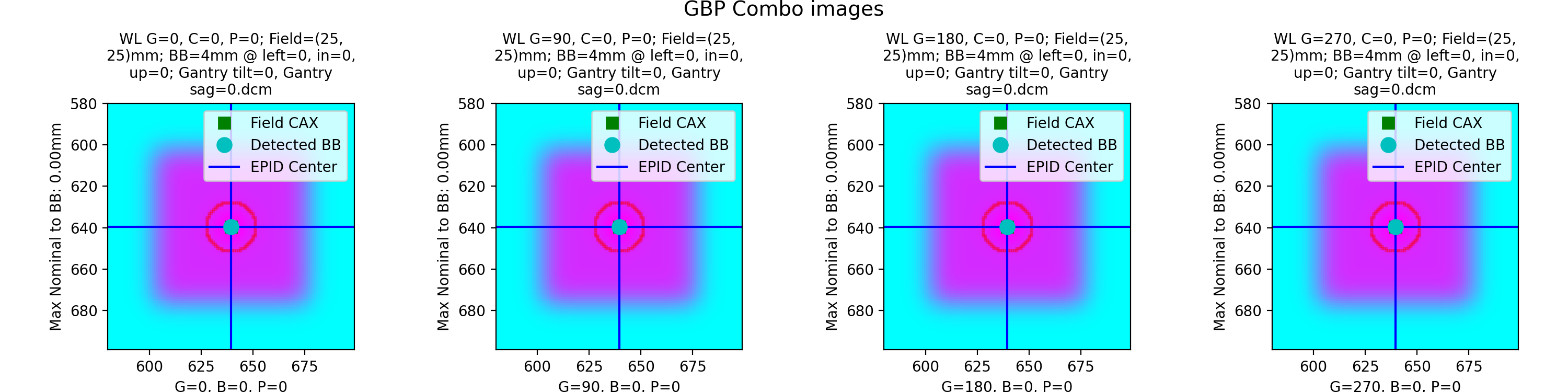
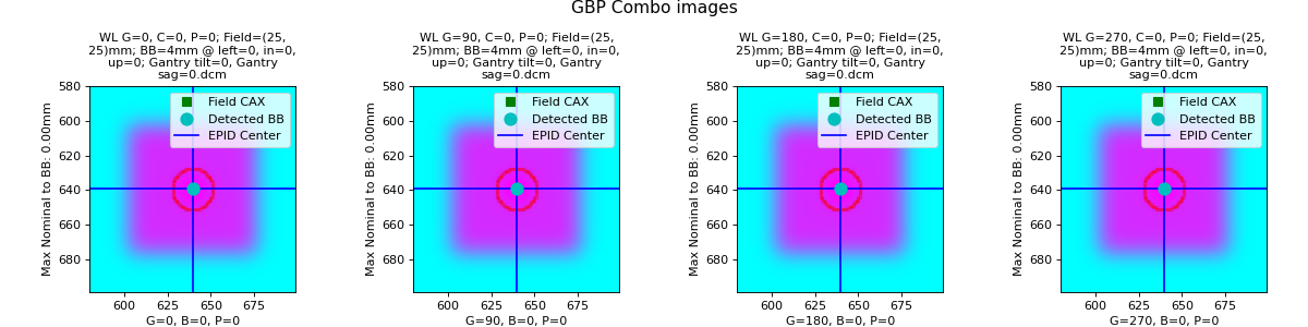
Let’s deliver a set of perfect images. This should result in near-0 deviations and isocenter size. The utility function used here will produce 4 images at the 4 cardinal gantry angles with all other axes at 0, with a BB of 4mm diameter, and a field size of 4x4cm:

import pylinac
from pylinac.winston_lutz import Axis
from pylinac.core.image_generator import (
    GaussianFilterLayer,
    FilteredFieldLayer,
    AS1200Image,
    RandomNoiseLayer,
    generate_winstonlutz,
)

wl_dir = 'wl_dir'
generate_winstonlutz(
    AS1200Image(1000),
    FilteredFieldLayer,
    dir_out=wl_dir,
    final_layers=[GaussianFilterLayer(),],
    bb_size_mm=4,
    field_size_mm=(25, 25),
)

wl = pylinac.WinstonLutz(wl_dir)
wl.analyze(bb_size_mm=4)
wl.plot_images(axis=Axis.GBP_COMBO)

(Source code, png, hires.png, pdf)

which has an output of:

Winston-Lutz Analysis
=================================
Number of images: 4
Maximum 2D CAX->BB distance: 0.00mm
Median 2D CAX->BB distance: 0.00mm
Mean 2D CAX->BB distance: 0.00mm
Shift to iso: facing gantry, move BB: RIGHT 0.00mm; OUT 0.00mm; DOWN 0.00mm
Gantry 3D isocenter diameter: 0.00mm (4/4 images considered)
Maximum Gantry RMS deviation (mm): 0.00mm
Maximum EPID RMS deviation (mm): 0.00mm
Gantry+Collimator 3D isocenter diameter: 0.00mm (4/4 images considered)
Collimator 2D isocenter diameter: 0.00mm (1/4 images considered)
Maximum Collimator RMS deviation (mm): 0.00
Couch 2D isocenter diameter: 0.00mm (1/4 images considered)
Maximum Couch RMS deviation (mm): 0.00

As shown, we have perfect results.

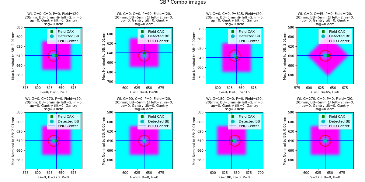
Offset BB¶

Let’s now offset the BB by 1mm to the left:

import pylinac
from pylinac.winston_lutz import Axis
from pylinac.core.image_generator import (
    GaussianFilterLayer,
    FilteredFieldLayer,
    AS1200Image,
    RandomNoiseLayer,
    generate_winstonlutz,
)

wl_dir = 'wl_dir_offset'
generate_winstonlutz(
    AS1200Image(1000),
    FilteredFieldLayer,
    dir_out=wl_dir,
    final_layers=[GaussianFilterLayer(),],
    bb_size_mm=4,
    field_size_mm=(25, 25),
    offset_mm_left=1,
)

wl = pylinac.WinstonLutz(wl_dir)
wl.analyze(bb_size_mm=4)
wl.plot_images(axis=Axis.GBP_COMBO)

(Source code, png, hires.png, pdf)

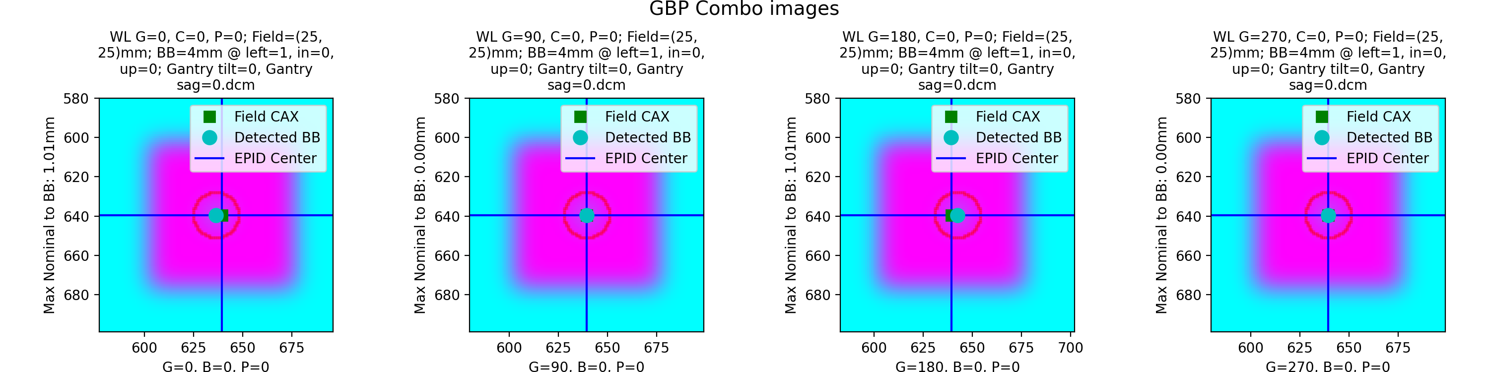
with an output of:

Winston-Lutz Analysis
=================================
Number of images: 4
Maximum 2D CAX->BB distance: 1.01mm
Median 2D CAX->BB distance: 0.50mm
Mean 2D CAX->BB distance: 0.50mm
Shift to iso: facing gantry, move BB: RIGHT 1.01mm; OUT 0.00mm; DOWN 0.00mm
Gantry 3D isocenter diameter: 0.00mm (4/4 images considered)
Maximum Gantry RMS deviation (mm): 1.01mm
Maximum EPID RMS deviation (mm): 0.00mm
Gantry+Collimator 3D isocenter diameter: 0.00mm (4/4 images considered)
Collimator 2D isocenter diameter: 0.00mm (1/4 images considered)
Maximum Collimator RMS deviation (mm): 0.00
Couch 2D isocenter diameter: 0.00mm (1/4 images considered)
Maximum Couch RMS deviation (mm): 0.00

We have correctly found that the max distance is 1mm and the required shift to iso is 1mm to the right (since we placed the bb to the left).

Gantry Tilt¶

Note

The term tilt (vs sag) here represents movement in the Y-axis coordinate space.

We can simulate gantry tilt, where at 0 and 180 the gantry tilts forward and backward respectively. We use a realistic value of 1mm. Note that everything else is perfect:

import pylinac
from pylinac.winston_lutz import Axis
from pylinac.core.image_generator import (
    GaussianFilterLayer,
    FilteredFieldLayer,
    AS1200Image,
    RandomNoiseLayer,
    generate_winstonlutz,
)

wl_dir = 'wl_dir_tilt'
generate_winstonlutz(
    AS1200Image(1000),
    FilteredFieldLayer,
    dir_out=wl_dir,
    final_layers=[GaussianFilterLayer(),],
    bb_size_mm=4,
    field_size_mm=(25, 25),
    gantry_tilt=1,
)

wl = pylinac.WinstonLutz(wl_dir)
wl.analyze(bb_size_mm=4)
wl.plot_images(axis=Axis.GBP_COMBO)

(Source code, png, hires.png, pdf)

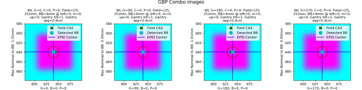
with output of:

Winston-Lutz Analysis
=================================
Number of images: 4
Maximum 2D CAX->BB distance: 1.01mm
Median 2D CAX->BB distance: 0.50mm
Mean 2D CAX->BB distance: 0.50mm
Shift to iso: facing gantry, move BB: RIGHT 0.00mm; OUT 0.00mm; DOWN 0.00mm
Gantry 3D isocenter diameter: 2.02mm (4/4 images considered)
Maximum Gantry RMS deviation (mm): 1.01mm
Maximum EPID RMS deviation (mm): 1.01mm
Gantry+Collimator 3D isocenter diameter: 2.02mm (4/4 images considered)
Collimator 2D isocenter diameter: 0.00mm (1/4 images considered)
Maximum Collimator RMS deviation (mm): 0.00
Couch 2D isocenter diameter: 0.00mm (1/4 images considered)
Maximum Couch RMS deviation (mm): 0.00

Note that since the tilt is symmetric the shift to iso is 0 despite our non-zero median distance. I.e. we are at iso, the iso just isn’t perfect and we are thus at the best possible position.

Gantry Sag¶

Note

The term sag (vs tilt) here represents movement in the Z-axis at 90/270 coordinate space.

We can simulate gantry sag, where at 90 and 270 the gantry tilts towards the floor. We use a realistic value of 1mm. Note that everything else is perfect:

import pylinac
from pylinac.winston_lutz import Axis
from pylinac.core.image_generator import (
    GaussianFilterLayer,
    FilteredFieldLayer,
    AS1200Image,
    RandomNoiseLayer,
    generate_winstonlutz,
)

wl_dir = 'wldir_sag'
generate_winstonlutz(
    AS1200Image(1000),
    FilteredFieldLayer,
    dir_out=wl_dir,
    final_layers=[GaussianFilterLayer(),],
    bb_size_mm=4,
    field_size_mm=(25, 25),
    gantry_sag=1,
)

wl = pylinac.WinstonLutz(wl_dir)
wl.analyze(bb_size_mm=4)
wl.plot_images(axis=Axis.GBP_COMBO)

(Source code, png, hires.png, pdf)

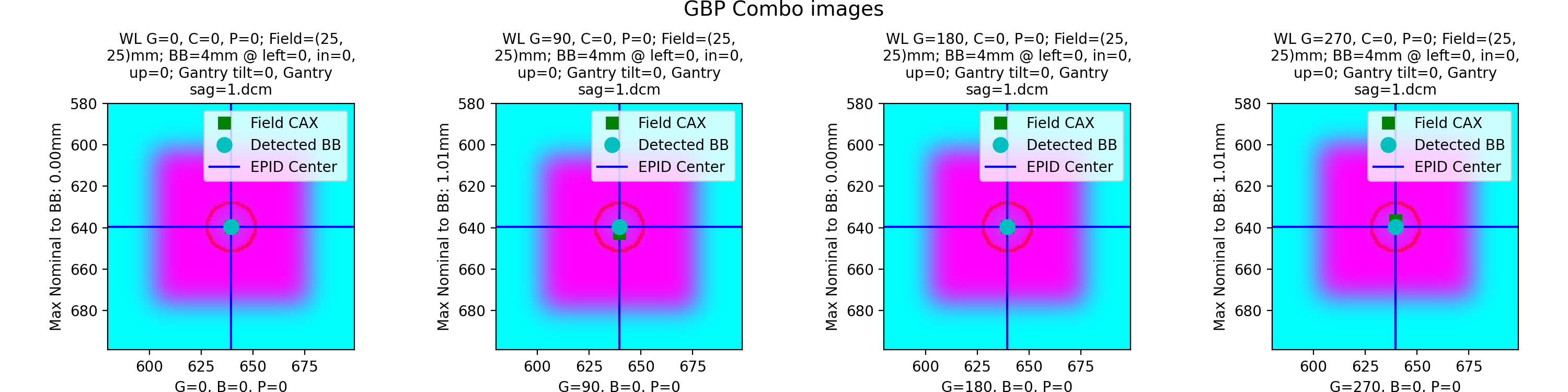
with output of:

Winston-Lutz Analysis
=================================
Number of images: 4
Maximum 2D CAX->BB distance: 1.01mm
Median 2D CAX->BB distance: 0.50mm
Mean 2D CAX->BB distance: 0.50mm
Shift to iso: facing gantry, move BB: LEFT 0.00mm; IN 0.00mm; DOWN 1.01mm
Gantry 3D isocenter diameter: 0.00mm (4/4 images considered)
Maximum Gantry RMS deviation (mm): 1.01mm
Maximum EPID RMS deviation (mm): 1.01mm
Gantry+Collimator 3D isocenter diameter: 0.00mm (4/4 images considered)
Collimator 2D isocenter diameter: 0.00mm (1/4 images considered)
Maximum Collimator RMS deviation (mm): 0.00
Couch 2D isocenter diameter: 0.00mm (1/4 images considered)
Maximum Couch RMS deviation (mm): 0.00

Sag will not realistically vary smoothly with gantry angle but for the purposes of the test it is a good approximation. This appears as an offset of the BB in the Z-axis.

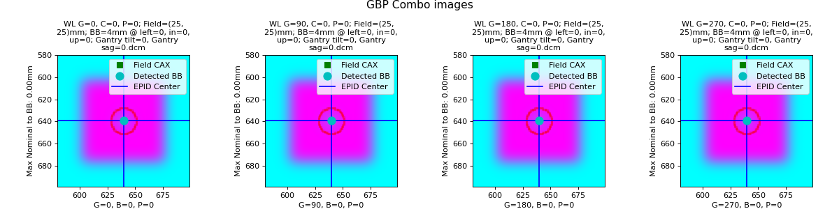
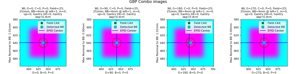
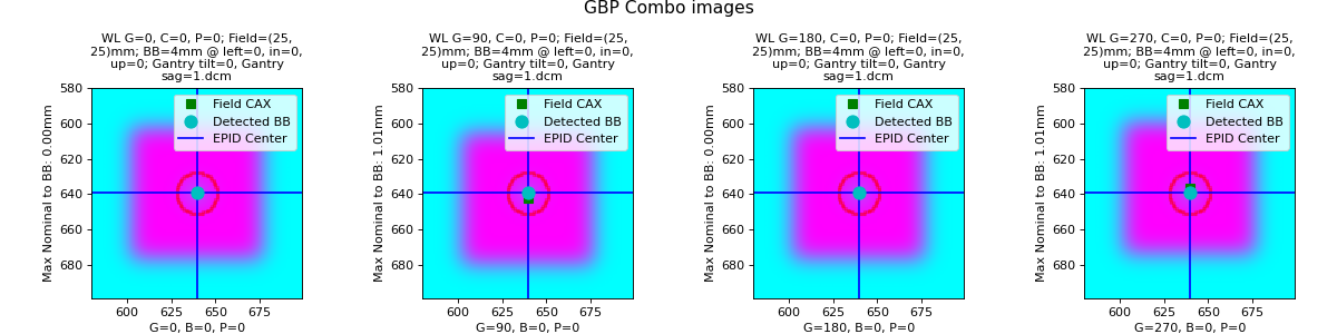
Offset Multi-Axis¶

We can also vary the axis data for the images produced. Below we create a typical multi-axis WL with varying gantry, collimator, and couch values. We offset the BB to the left by 2mm for visualization purposes:

import pylinac
from pylinac.winston_lutz import Axis
from pylinac.core.image_generator import (
    GaussianFilterLayer,
    FilteredFieldLayer,
    AS1200Image,
    RandomNoiseLayer,
    generate_winstonlutz,
)

wl_dir = 'wl_dir_offset_multi'
generate_winstonlutz(
    AS1200Image(1000),
    FilteredFieldLayer,
    dir_out=wl_dir,
    final_layers=[GaussianFilterLayer(sigma_mm=1), ],
    bb_size_mm=5,
    field_size_mm=(20, 20),
    offset_mm_left=2,
    image_axes=[(0, 0, 0), (0, 45, 0), (0, 270, 0),
                (90, 0, 0), (180, 0, 0), (270, 0, 0),
                (0, 0, 90), (0, 0, 315)]
)

wl = pylinac.WinstonLutz(wl_dir)
wl.analyze(bb_size_mm=5)
print(wl.results())
wl.plot_images(axis=Axis.GBP_COMBO)

(Source code, png, hires.png, pdf)

with output of:

Winston-Lutz Analysis
=================================
Number of images: 8
Maximum 2D CAX->BB distance: 2.01mm
Median 2D CAX->BB distance: 2.01mm
Mean 2D CAX->BB distance: 1.51mm
Shift to iso: facing gantry, move BB: RIGHT 2.01mm; OUT 0.00mm; DOWN 0.00mm
Gantry 3D isocenter diameter: 0.00mm (4/8 images considered)
Maximum Gantry RMS deviation (mm): 2.01mm
Maximum EPID RMS deviation (mm): 0.00mm
Gantry+Collimator 3D isocenter diameter: 0.00mm (6/8 images considered)
Collimator 2D isocenter diameter: 0.00mm (3/8 images considered)
Maximum Collimator RMS deviation (mm): 2.01
Couch 2D isocenter diameter: 3.72mm (3/8 images considered)
Maximum Couch RMS deviation (mm): 2.01

Note the shift to iso is 2mm to the right, as we offset the BB to the left by 2mm, even with our couch kicks and collimator rotations.

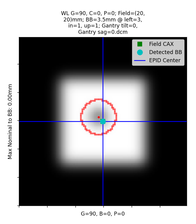
Perfect Cone¶

We can also look at simulated cone WL images. Here we use the 17.5mm cone:

import pylinac
from pylinac.winston_lutz import Axis
from pylinac.core.image_generator import (
    GaussianFilterLayer,
    FilteredFieldLayer,
    AS1200Image,
    RandomNoiseLayer,
    generate_winstonlutz, generate_winstonlutz_cone, FilterFreeConeLayer,
)

wl_dir = 'wl_dir_cone'
generate_winstonlutz_cone(
    AS1200Image(1000),
    FilterFreeConeLayer,
    dir_out=wl_dir,
    final_layers=[GaussianFilterLayer(), ],
    bb_size_mm=4,
    cone_size_mm=17.5,
)

wl = pylinac.WinstonLutz(wl_dir)
wl.analyze(bb_size_mm=4)
print(wl.results())
wl.plot_images(axis=Axis.GBP_COMBO)

(Source code, png, hires.png, pdf)

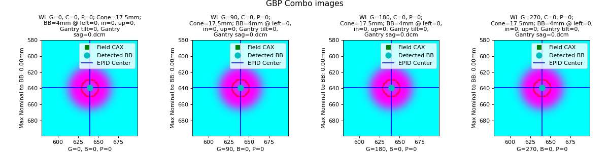
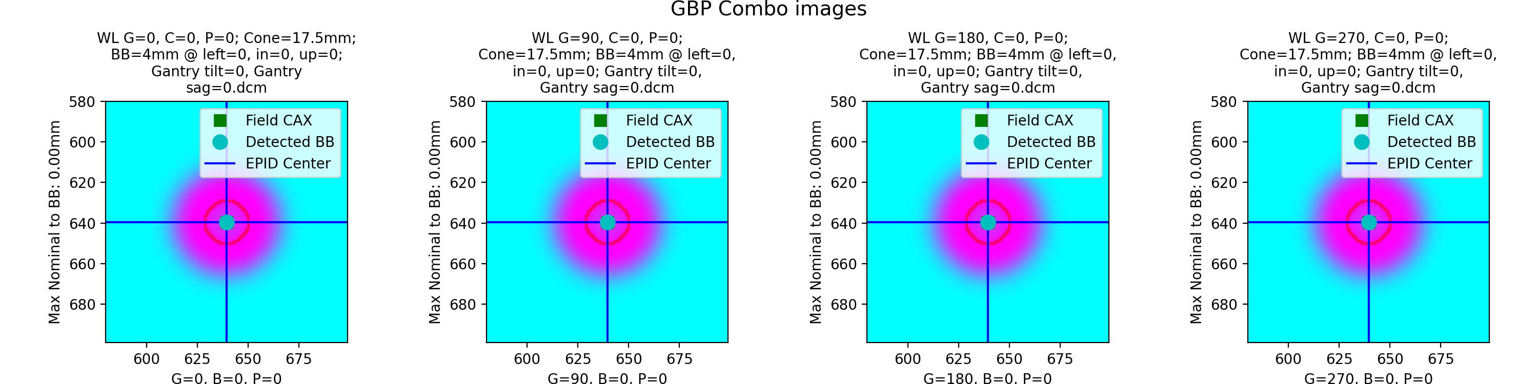
Low-density BB¶

Simulate a low-density BB surrounded by higher-density material:

import pylinac
from pylinac.winston_lutz import Axis
from pylinac.core.image_generator import (
    GaussianFilterLayer,
    FilteredFieldLayer,
    AS1200Image,
    RandomNoiseLayer,
    generate_winstonlutz,
)

wl_dir = 'wl_dir_low'
generate_winstonlutz(
    AS1200Image(1000),
    FilteredFieldLayer,
    dir_out=wl_dir,
    final_layers=[GaussianFilterLayer(), ],
    bb_size_mm=4,
    field_size_mm=(25, 25),
    field_alpha=0.6,  # set the field to not max out
    bb_alpha=0.3  # normally this is negative to attenuate the beam, but here we increase the signal
)

wl = pylinac.WinstonLutz(wl_dir)
wl.analyze(bb_size_mm=4, low_density_bb=True)
print(wl.results())
wl.plot_images(axis=Axis.GBP_COMBO)

(Source code, png, hires.png, pdf)

API Documentation¶

Bases: ResultsDataMixin[WinstonLutzResult], QuaacMixin

Class for performing a Winston-Lutz test of the radiation isocenter.

Parameters¶

directorystr, list[str]: Path to the directory of the Winston-Lutz EPID images or a list of the image paths
use_filenames: bool: Whether to try to use the file name to determine axis values. Useful for Elekta machines that do not include that info in the DICOM data. This is mutually exclusive to axis_mapping. If True, axis_mapping is ignored.
axis_mapping: dict: An optional way of instantiating by passing each file along with the axis values. Structure should be <filename>: (<gantry>, <coll>, <couch>).
axes_precision: int | None: How many significant digits to represent the axes values. If None, no precision is set and the input/DICOM values are used raw. If set to an integer, rounds the axes values (gantry, coll, couch) to that many values. E.g. gantry=0.1234 => 0.1 with precision=1. This is mostly useful for plotting/rounding (359.9=>0) and if using the keyed_image_details with results_data.
dpi: The dots-per-inch setting. Only needed if using TIFF images and the images do not contain the resolution tag. An error will raise if dpi is not passed and the TIFF resolution cannot be determined.
sid: The Source-to-Image distance in mm. Only needed when using TIFF images.

machine_scale: MachineScale¶

image_type¶: alias of WinstonLutz2D

images: list[WinstonLutz2D]¶

classmethod from_demo_images(**kwargs)[source]¶

Instantiate using the demo images.

Parameters¶

kwargs: See parameters of the __init__ method for details.

classmethod from_zip(zfile: str | BinaryIO | Path, **kwargs)[source]¶

Instantiate from a zip file rather than a directory.

Parameters¶

zfile: Path to the archive file.
kwargs: See parameters of the __init__ method for details.

classmethod from_url(url: str, **kwargs)[source]¶

Instantiate from a URL.

Parameters¶

urlstr: URL that points to a zip archive of the DICOM images.
kwargs: See parameters of the __init__ method for details.

classmethod from_cbct_zip(file: Path | str, raw_pixels: bool = False, **kwargs)[source]¶

Instantiate from a zip file containing CBCT images.

Parameters¶

file: Path to the archive file.
raw_pixels: If True, uses the raw pixel values of the DICOM files. If False, uses the rescaled Hounsfield units. Generally, this should be true.
kwargs: See parameters of the __init__ method for details.

classmethod from_cbct(directory: Path | str, raw_pixels: bool = False, **kwargs)[source]¶

Create a 4-angle WL test from a CBCT dataset.

The dataset is loaded and the array is “viewed” from top, bottom, left, and right to create the 4 angles. The dataset has to be rescaled so that the z-axis spacing is equal to the x/y axis. This is because the typical slice thickness is much larger than the in-plane resolution.

Parameters¶

directory: The directory containing the CBCT DICOM files.
raw_pixels: If True, uses the raw pixel values of the DICOM files. If False, uses the rescaled Hounsfield units. Generally, this should be true.
kwargs: See parameters of the __init__ method for details.

static run_demo() → None[source]¶: Run the Winston-Lutz demo, which loads the demo files, prints results, and plots a summary image.

analyze(bb_size_mm: float = 5, machine_scale: MachineScale = MachineScale.IEC61217, low_density_bb: bool = False, open_field: bool = False, apply_virtual_shift: bool = False, snap_tolerance: float = 3, gantry_reference: float = 0, collimator_reference: float = 0, couch_reference: float = 0, bb_proximity_mm: float = 20) → None[source]¶

Analyze the WL images.

Parameters¶

bb_size_mm: The expected diameter of the BB in mm. The actual size of the BB can be +/-2mm from the passed value.
machine_scale: The scale of the machine. Shift vectors depend on this value.
low_density_bb: Set this flag to True if the BB is lower density than the material surrounding it.
open_field: If True, sets the field center to the EPID center under the assumption the field is not the focus of interest or is too wide to be calculated. This is often helpful for kV WL analysis where the blades are wide open and even then the blade edge is of less interest than simply the imaging iso vs the BB.
apply_virtual_shift: If True, applies a virtual shift to the BBs based on the shift necessary to place the BB at the radiation isocenter.
snap_tolerance: The tolerance of the axes values that will “snap” to the reference values. I.e. if the snap tolerance is 3 and the gantry is within 3 degrees of 0, it will snap to 0. This is helpful, e.g., when you’ve forgotten to reset the couch to 0 after a CBCT.
gantry_reference: The reference value for the gantry. This is when pylinac will consider the image to be a reference image. E.g. some customers take all images with collimator=45 and want that to be considered the reference. This is used in combination with the snap_tolerance. I.e. a gantry of 43 with snap tolerance of 3 and reference of 45 will snap to 45.
collimator_reference: The reference value for the collimator. See gantry_reference.
couch_reference: The reference value for the couch. See gantry_reference.
bb_proximity_mm: The maximum distance in mm that a detected BB can be from the expected BB position. For single-BB WL datasets, the expected BB position is isocenter.

property gantry_iso_size: float¶: The diameter of the 3D gantry isocenter size in mm. Only images where the collimator and couch were at 0 are used to determine this value.

property gantry_coll_iso_size: float¶: The diameter of the 3D gantry isocenter size in mm including collimator and gantry/coll combo images. Images where the couch!=0 are excluded.

property collimator_iso_size: float¶: The 2D collimator isocenter size (diameter) in mm. The iso size is in the plane normal to the gantry.

property couch_iso_size: float¶: The diameter of the 2D couch isocenter size in mm. Only images where the gantry and collimator were at zero are used to determine this value.

property bb_shift_vector: Vector¶

The shift necessary to place the BB at the radiation isocenter. The values are in the coordinates defined in the documentation.

The shift is based on the paper by Low et al. See online documentation and the solve_3d_shift_vector_from_2d_planes function for more., which is how the measured bb and field positions are determined.

bb_shift_instructions(couch_vrt: float | None = None, couch_lng: float | None = None, couch_lat: float | None = None) → str[source]¶

Returns a string describing how to shift the BB to the radiation isocenter looking from the foot of the couch. Optionally, the current couch values can be passed in to get the new couch values. If passing the current couch position all values must be passed.

Parameters¶

couch_vrtfloat: The current couch vertical position in cm.
couch_lngfloat: The current couch longitudinal position in cm.
couch_latfloat: The current couch lateral position in cm.

axis_rms_deviation(axis: Axis | tuple[Axis, ...] = Axis.GANTRY, value: str = 'all') → Iterable | float[source]¶

The RMS deviations of a given axis/axes.

Parameters¶

axis(‘Gantry’, ‘Collimator’, ‘Couch’, ‘Epid’, ‘GB Combo’, ‘GBP Combo’): The axis desired.
value{‘all’, ‘range’}: Whether to return all the RMS values from all images for that axis, or only return the maximum range of values, i.e. the ‘sag’.

cax2bb_distance(metric: str = 'max') → float[source]¶

The distance in mm between the CAX and BB for all images according to the given metric.

Parameters¶

metric{‘max’, ‘median’, ‘mean’}: The metric of distance to use.

cax2epid_distance(metric: str = 'max') → float[source]¶

The distance in mm between the CAX and EPID center pixel for all images according to the given metric.

Parameters¶

metric{‘max’, ‘median’, ‘mean’}: The metric of distance to use.

plotly_analyzed_images(zoomed: bool = True, show_legend: bool = True, show: bool = True, show_colorbar: bool = True, **kwargs) → dict[str, Figure][source]¶

Plot the analyzed images in a Plotly figure.

Parameters¶

zoomedbool: Whether to zoom in on the BBs of the 2D images.
show_legendbool: Whether to show the legend on the plot.
showbool: Whether to show the plot.
show_colorbarbool: Whether to show the colorbar on the plot.
kwargs: Additional keyword arguments to pass to the plot.

Returns¶

dict: A dictionary of the Plotly figures where the key is the name of the image and the value is the figure.

plot_axis_images(axis: Axis = Axis.GANTRY, show: bool = True, ax: Axes | None = None) → None[source]¶

Plot all CAX/BB/EPID positions for the images of a given axis.

For example, axis=’Couch’ plots a reference image, and all the BB points of the other images where the couch was moving.

Parameters¶

axis{‘Gantry’, ‘Collimator’, ‘Couch’, ‘GB Combo’, ‘GBP Combo’}: The images/markers from which accelerator axis to plot.
showbool: Whether to actually show the images.
axNone, matplotlib.Axes: The axis to plot to. If None, creates a new plot.

plot_location(show: bool = True, viewbox_mm: float | None = None, plot_bb: bool = True, plot_isocenter_sphere: bool = True, plot_couch_iso: bool = True, plot_coll_iso: bool = True, show_legend: bool = True)[source]¶

Plot the isocenter and size as a sphere in 3D space relative to the BB. The iso is at the origin.

Only images where the couch was at zero are considered.

Parameters¶

showbool: Whether to plot the image.
viewbox_mmfloat: The default size of the 3D space to plot in mm in each axis.
plot_bbbool: Whether to plot the BB location; the size is also considered.
plot_isocenter_spherebool: Whether to plot the gantry + collimator isocenter size.
plot_couch_isobool: Whether to plot the couch-plane-only isocenter size. This will be zero if there are no images where the couch rotated.
plot_coll_isobool: Whether to plot the collimator-plane-only isocenter size. This is shown along the Z/Y plane only to differentiate from the couch iso visualization. The collimator plane is always normal to the gantry angle. This will be zero if there are no images where the collimator rotated.
show_legendbool: Whether to show the legend.

plot_images(axis: Axis = Axis.GANTRY, show: bool = True, zoom: bool = True, legend: bool = True, split: bool = False, **kwargs)[source]¶

Plot a grid of all the images acquired.

Four columns are plotted with the titles showing which axis that column represents.

Parameters¶

axis{‘Gantry’, ‘Collimator’, ‘Couch’, ‘GB Combo’, ‘GBP Combo’, ‘All’}: The axis to plot.
showbool: Whether to show the image.
zoombool: Whether to zoom in around the BB.
legendbool: Whether to show the legend.
splitbool: Whether to show/plot the images individually or as one large figure.

save_images(filename: str | BinaryIO, axis: Axis = Axis.GANTRY, **kwargs) → None[source]¶

Save the figure of plot_images() to file. Keyword arguments are passed to matplotlib.pyplot.savefig().

Parameters¶

filenamestr: The name of the file to save to.
axis: The axis to save.

save_images_to_stream(**kwargs) → dict[str, BytesIO][source]¶: Save the individual image plots to stream

plot_summary(show: bool = True, fig_size: tuple | None = None) → None[source]¶: Plot a summary figure showing the gantry sag and wobble plots of the three axes.

save_summary(filename: str | BinaryIO, **kwargs) → None[source]¶: Save the summary image.

results(as_list: bool = False) → str[source]¶

Return the analysis results summary.

Parameters¶

as_listbool: Whether to return as a list of strings vs single string. Pretty much for internal usage.

Publish (print) a PDF containing the analysis, images, and quantitative results.

Parameters¶

filename(str, file-like object}: The file to write the results to.
notesstr, list of strings: Text; if str, prints single line. If list of strings, each list item is printed on its own line.
open_filebool: Whether to open the file using the default program after creation.
metadatadict: Extra data to be passed and shown in the PDF. The key and value will be shown with a colon. E.g. passing {‘Author’: ‘James’, ‘Unit’: ‘TrueBeam’} would result in text in the PDF like: ————– Author: James Unit: TrueBeam ————–
logo: Path, str: A custom logo to use in the PDF report. If nothing is passed, the default pylinac logo is used.

clear_captured_warnings() → None¶: Clear the list of captured warnings.

get_captured_warnings() → list[dict]¶: Retrieve the list of captured warnings, deduplicated.

results_data(as_dict: bool = False, as_json: bool = False, by_alias: bool = False, exclude: set[str] | None = None) → T | dict | str¶

Present the results data and metadata as a dataclass, dict, or tuple. The default return type is a dataclass.

Parameters¶

as_dictbool: If True, return the results as a dictionary.
as_jsonbool: If True, return the results as a JSON string. Cannot be True if as_dict is True.
by_aliasbool: If True, use the alias names of the dataclass fields. These are generally the more human-readable names.
excludeset: A set of fields to exclude from the results data.

to_quaac(path: str | Path, performer: User, primary_equipment: Equipment, format: Literal['json', 'yaml'] = 'yaml', attachments: list[Attachment] | None = None, overwrite: bool = False, **kwargs) → None¶

Write an analysis to a QuAAC file. This will include the items from results_data() and the PDF report.

Parameters¶

pathstr, Path: The file to write the results to.
performerUser: The user who performed the analysis.
primary_equipmentEquipment: The equipment used in the analysis.
format{‘json’, ‘yaml’}: The format to write the file in.
attachmentslist of Attachment: Additional attachments to include in the QuAAC file.
overwritebool: Whether to overwrite the file if it already exists.
kwargs: Additional keyword arguments to pass to the Document instantiation.

pydantic model pylinac.winston_lutz.WinstonLutzResult[source]¶

Bases: ResultBase

This class should not be called directly. It is returned by the results_data() method. It is a dataclass under the hood and thus comes with all the dunder magic.

Use the following attributes as normal class attributes.

Create a new model by parsing and validating input data from keyword arguments.

Raises [ValidationError][pydantic_core.ValidationError] if the input data cannot be validated to form a valid model.

self is explicitly positional-only to allow self as a field name.

field max_2d_cax_to_bb_mm: float [Required]¶: The maximum 2D distance from the field CAX to the BB across all images analyzed in mm.

field median_2d_cax_to_bb_mm: float [Required]¶: The median 2D distance from the field CAX to the BB across all images analyzed in mm.

field mean_2d_cax_to_bb_mm: float [Required]¶: The mean 2D distance from the field CAX to the BB across all images analyzed in mm.

field max_2d_cax_to_epid_mm: float [Required]¶: The maximum 2D distance from the field CAX to the EPID center across all images analyzed in mm.

field median_2d_cax_to_epid_mm: float [Required]¶: The median 2D distance from the field CAX to the EPID center across all images analyzed in mm.

field mean_2d_cax_to_epid_mm: float [Required]¶: The mean 2D distance from the field CAX to the EPID center across all images analyzed in mm.

field gantry_3d_iso_diameter_mm: float [Required]¶: The 3D isocenter diameter of the gantry axis only as determined by the gantry images in mm. This uses backprojection lines of the field center to the source and minimizes a sphere that touches all the backprojection lines.

field coll_2d_iso_diameter_mm: float [Required]¶: The 2D isocenter diameter of the collimator axis only as determined by the collimator images in mm.

field couch_2d_iso_diameter_mm: float [Required]¶: The 2D isocenter diameter of the couch axis only as determined by the couch images in mm.

field gantry_coll_3d_iso_diameter_mm: float [Required]¶: The 3D isocenter diameter of the gantry and collimator axes as determined by the gantry and collimator images in mm.

field num_total_images: int [Required]¶: The total number of images analyzed.

field num_gantry_images: int [Required]¶: The number of images that were taken at different gantry angles and all other axes were at reference.

field num_coll_images: int [Required]¶: The number of images that were taken at different collimator angles and all other axes were at reference.

field num_couch_images: int [Required]¶: The number of images that were taken at different couch angles and all other axes were at reference.

field num_gantry_coll_images: int [Required]¶: The number of images that were taken at different gantry and collimator angles and the couch was at reference.

field max_gantry_rms_deviation_mm: float [Required]¶: The maximum RMS value of the field CAX to BB for the gantry axis images in mm. This is an alternative to the max/mean/median calculations.

field max_epid_rms_deviation_mm: float [Required]¶: The maximum RMS value of the field CAX to EPID center for the EPID images in mm. This is an alternative to the max/mean/median calculations.

field max_coll_rms_deviation_mm: float [Required]¶: The maximum RMS deviation of the field CAX to BB for the collimator axis images in mm. This is an alternative to the max/mean/median calculations.

field max_couch_rms_deviation_mm: float [Required]¶: The maximum RMS value of the field CAX to BB for the couch axis images in mm. This is an alternative to the max/mean/median calculations. This uses backprojection lines of the field center to the source and minimizes a sphere that touches all the backprojection lines.

field bb_shift_vector: VectorSerialized [Required]¶: The Cartesian vector that would move the BB to the radiation isocenter. Each value is in mm.

field image_details: list[WinstonLutz2DResult] [Required]¶: A list of the individual image results.

field keyed_image_details: dict[str, WinstonLutz2DResult] [Required]¶: A dictionary of the individual image results. This is the same as image_details but keyed by the images using the axes values as the key. E.g. G0B45P0. This can be used to identify individual images vs those in image_details.

class pylinac.winston_lutz.WinstonLutz2D(file: str | BinaryIO | Path, use_filenames: bool = False, **kwargs)[source]¶

Bases: WLBaseImage, ResultsDataMixin[WinstonLutz2DResult]

Holds individual Winston-Lutz EPID images, image properties, and automatically finds the field CAX and BB.

Parameters¶

filestr: Path to the image file.
use_filenames: bool: Whether to try to use the file name to determine axis values. Useful for Elekta machines that do not include that info in the DICOM data.

analyze(bb_size_mm: float = 5, low_density_bb: bool = False, open_field: bool = False, shift_vector: Vector | None = None, snap_tolerance: float = 3, gantry_reference: float = 0, collimator_reference: float = 0, couch_reference: float = 0, bb_proximity_mm: float = 20, machine_scale: MachineScale = MachineScale.IEC61217) → None[source]¶: Analyze the image. See WinstonLutz.analyze for parameter details.

property cax2bb_vector: Vector¶: The vector in mm from the CAX to the BB.

property cax2bb_distance: float¶: The scalar distance in mm from the CAX to the BB.

property cax2epid_vector: Vector¶: The vector in mm from the CAX to the EPID center pixel

property cax2epid_distance: float¶: The scalar distance in mm from the CAX to the EPID center pixel

save_plot(filename: str, **kwargs)[source]¶: Save the image plot to file.

as_binary(threshold: int) → DicomImage | ArrayImage | FileImage | LinacDicomImage¶

Return a binary (black & white) image based on the given threshold.

Parameters¶

thresholdint, float: The threshold value. If the value is above or equal to the threshold it is set to 1, otherwise to 0.

Returns¶

ArrayImage

as_dicom(gantry: float, coll: float, couch: float, extra_tags: dict | None = None) → Dataset¶: Convert the array to a DICOM file.

bit_invert() → None¶: Invert the image bit-wise

check_inversion(box_size: int = 20, position: float, float = (0.0, 0.0)) → None¶

Check the image for inversion by sampling the 4 image corners. If the average value of the four corners is above the average pixel value, then it is very likely inverted.

Parameters¶

box_sizeint: The size in pixels of the corner box to detect inversion.
position2-element sequence: The location of the sampling boxes.

check_inversion_by_histogram(percentiles: float, float, float = (5, 50, 95)) → bool¶

Check the inversion of the image using histogram analysis. The assumption is that the image is mostly background-like values and that there is a relatively small amount of dose getting to the image (e.g. a picket fence image). This function looks at the distance from one percentile to another to determine if the image should be inverted.

Parameters¶

percentiles3-element tuple: The 3 percentiles to compare. Default is (5, 50, 95). Recommend using (x, 50, y). To invert the other way (where pixel value is decreasing with dose, reverse the percentiles, e.g. (95, 50, 5).

Returns¶

bool: Whether an inversion was performed.

clear_captured_warnings() → None¶: Clear the list of captured warnings.

compute(metrics: list[MetricBase] | MetricBase) → Any | dict[str, Any]¶

Compute the given metrics on the image.

This can be called multiple times to compute different metrics. Metrics are appended on each call. This allows for modification of the image between metric calls as well as the ability to compute different metrics on the same image that might depend on earlier metrics.

Metrics are both returned and stored in the metrics attribute. The metrics attribute will store all metrics every calculated. The metrics returned are only those passed in the metrics argument.

Parameters¶

metricslist[MetricBase] | MetricBase: The metric(s) to compute.

crop(pixels: int = 15, edges: tuple[str, ...] = ('top', 'bottom', 'left', 'right')) → None¶

Removes pixels on all edges of the image in-place.

Parameters¶

pixelsint: Number of pixels to cut off all sides of the image.
edgestuple: Which edges to remove from. Can be any combination of the four edges.

date_created(format: str = '%A, %B %d, %Y') → str¶

The date the file was created. Tries DICOM data before falling back on OS timestamp. The method use one or more inputs of formatted code, where % means a placeholder and the letter the time unit of interest. For a full description of the several formatting codes see strftime() documentation.

Parameters¶

formatstr: %A means weekday full name, %B month full name, %d day of the month as a zero-padded decimal number and %Y year with century as a decimal number.

Returns¶

str: The date the file was created.

dist2edge_min(point: Point | tuple) → float¶: Calculates distance from given point to the closest edge.

Parameters¶

point : geometry.Point, tuple

Returns¶

float

epid_to_bb_distances() → list[float]¶: The distances from the EPID center to the BBs in mm. Useful for metrics as this is only the resulting floats vs a dict of points.

field_to_bb_distances() → list[float]¶: The distances from the field CAXs to the BBs in mm. Useful for metrics as this is only the resulting floats vs a dict of points.

filter(size: float | int = 0.05, kind: str = 'median') → None¶

Filter the profile in place.

Parameters¶

sizeint, float: Size of the median filter to apply. If a float, the size is the ratio of the length. Must be in the range 0-1. E.g. if size=0.1 for a 1000-element array, the filter will be 100 elements. If an int, the filter is the size passed.
kind{‘median’, ‘gaussian’}: The kind of filter to apply. If gaussian, size is the sigma value.

find_bb_centroids(bb_diameter_mm: float, low_density: bool) → list[Point]¶: Find BBs in the image. This method can return MORE than the desired number of BBs. Matching of the detected BBs vs the expected BBs is done in the find_bb_matches method.

find_bb_matches(detected_points: list[Point], bb_proximity_mm: float) → dict[str, Point]¶

Given an arrangement and detected BB positions, find the bbs that are closest to the expected positions.

This is to prevent false positives from being detected as BBs (e.g. noise, couch, etc). The detected BBs are matched to the expected BBs based on proximity.

These matches are linked to the individual BB arrangement by arrangement name.

find_field_centroids(is_open_field: bool) → list[Point]¶: Find the field CAX(s) in the image. If the field is open or this is a vanilla WL, only one CAX is found.

find_field_matches(detected_points: list[Point], bb_proximity_mm: float) → dict[str, Point]¶: Find matches between detected field points and the arrangement. See find_bb_matches for more info.

fliplr() → None¶: Flip the image array upside down in-place. Wrapper for np.fliplr()

flipud() → None¶: Flip the image array upside down in-place. Wrapper for np.flipud()

gamma(comparison_image: DicomImage | ArrayImage | FileImage | LinacDicomImage, doseTA: float = 1, distTA: float = 1, threshold: float = 0.1, ground: bool = True, normalize: bool = True) → ndarray¶

Calculate the gamma between the current image (reference) and a comparison image.

Added in version 1.2.

The gamma calculation is based on Bakai et al eq.6, which is a quicker alternative to the standard Low gamma equation.

Parameters¶

comparison_image{ArrayImage, DicomImage, or FileImage}: The comparison image. The image must have the same DPI/DPMM to be comparable. The size of the images must also be the same.
doseTAint, float: Dose-to-agreement in percent; e.g. 2 is 2%.
distTAint, float: Distance-to-agreement in mm.
thresholdfloat: The dose threshold percentage of the maximum dose, below which is not analyzed. Must be between 0 and 1.
groundbool: Whether to “ground” the image values. If true, this sets both datasets to have the minimum value at 0. This can fix offset errors in the data.
normalizebool: Whether to normalize the images. This sets the max value of each image to the same value.

Returns¶

gamma_mapnumpy.ndarray: The calculated gamma map.

Returns¶

float: The amount subtracted from the image.

invert() → None¶: Invert (imcomplement) the image.

nominal_bb_position(bb_config: BBConfig) → Point¶: Calculate the expected point position in 2D

normalize(norm_val: str | float | None = None) → None¶

Normalize the profile to the given value.

Parameters¶

valuenumber or None: If a number, normalize the array to that number. If None, normalizes to the maximum value.

plot(ax: Axes | None = None, show: bool = True, clear_fig: bool = False, zoom: bool = True, legend: bool = True, **kwargs) → Axes¶

Plot an individual WL image.

Parameters¶

axNone, plt.Axes: The axis to plot to. If None, a new figure is created.
showbool: Whether to show the plot.
clear_figbool: Whether to clear the figure before plotting.
zoombool: Whether to zoom in on the BBs. If False, no zooming is done and the entire image is shown.
legendbool: Whether to show the legend.

plot_metrics(show: bool = True) → list[figure]¶

Plot any additional figures from the metrics.

Returns a list of figures of the metrics. These metrics are not drawn on the original image but rather are something complete separate. E.g. a profile plot or a histogram of the metric.

plotly(fig: Figure | None = None, show: bool = True, zoomed: bool = True, show_legend: bool = True, show_colorbar: bool = True) → Figure¶

Plot the image with the detected BB, outlines, and field CAX.

Parameters¶

fig: go.Figure, None: The Plotly figure
show: Whether to show the plot
zoomed: Whether to zoom in on the BBs. If False, no zooming is done and the entire image is shown.
show_legend: Whether to show the legend.
show_colorbar: Whether to show the colorbar.

Returns¶

go.Figure

results_data(as_dict: bool = False, as_json: bool = False, by_alias: bool = False, exclude: set[str] | None = None) → T | dict | str¶

Present the results data and metadata as a dataclass, dict, or tuple. The default return type is a dataclass.

Parameters¶

as_dictbool: If True, return the results as a dictionary.
as_jsonbool: If True, return the results as a JSON string. Cannot be True if as_dict is True.
by_aliasbool: If True, use the alias names of the dataclass fields. These are generally the more human-readable names.
excludeset: A set of fields to exclude from the results data.

roll(direction: str = 'x', amount: int = 1) → None¶

Roll the image array around in-place. Wrapper for np.roll().

Parameters¶

direction{‘x’, ‘y’}: The axis to roll over.
amountint: The amount of elements to roll over.

rot90(n: int = 1) → None¶: Wrapper for numpy.rot90; rotate the array by 90 degrees CCW n times.

rotate(angle: float, mode: str = 'edge', *args, **kwargs)¶: Rotate the image counter-clockwise. Simple wrapper for scikit-image. See https://scikit-image.org/docs/stable/api/skimage.transform.html#skimage.transform.rotate. All parameters are passed to that function.

save(filename: str | Path) → str | Path¶

Save the image instance back out to a .dcm file.

Parameters¶

filenamestr, Path: The filename to save the DICOM file as.

Returns¶

A string pointing to the new filename.

threshold(threshold: float, kind: str = 'high') → None¶

Apply a high- or low-pass threshold filter.

Parameters¶

thresholdint: The cutoff value.
kindstr: If high (default), will apply a high-pass threshold. All values above the cutoff are left as-is. Remaining points are set to 0. If low, will apply a low-pass threshold.

to_axes() → str¶: Give just the axes values as a human-readable string

pydantic model pylinac.winston_lutz.WinstonLutz2DResult[source]¶

Bases: ResultBase

Create a new model by parsing and validating input data from keyword arguments.

Raises [ValidationError][pydantic_core.ValidationError] if the input data cannot be validated to form a valid model.

self is explicitly positional-only to allow self as a field name.

field variable_axis: str [Required]¶: The axis that varied in the image.

field bb_location: PointSerialized [Required]¶: The location of the BB in the image as a Point in pixels.

field cax2epid_vector: VectorSerialized [Required]¶: The vector (in Cartesian coordinates) from the field CAX to the EPID center in mm.

field cax2epid_distance: float [Required]¶: The distance from the field CAX to the EPID center in mm.

field cax2bb_vector: VectorSerialized [Required]¶: The vector (in Cartesian coordinates) from the field CAX to the BB in mm.

field cax2bb_distance: float [Required]¶: The scalar distance from the field CAX to the BB in mm.

field field_cax: PointSerialized [Required]¶: The location of the field CAX in the image as a Point in pixels.

Winston-Lutz¶

Overview¶

Running the Demo¶

Image Acquisition¶

Axis Values¶

Coordinate Space¶

Passing a coordinate system¶

Typical Use¶

Visualizing the Isocenter-to-BB¶

Accessing data¶

Accessing individual images¶

Analyzing a single image¶

Passing in Axis values¶

via filenames¶

via axis_mapping¶

Setting Reference Axis Values¶

Changing BB detection size¶

Low-density BBs¶

kV Analysis/Imaging-only iso evaluation¶

CBCT Analysis¶

Virtual Shifting¶

Using TIFF images¶

Image types & output definitions¶

Interpreting Results¶

Interpreting specific publications¶

Analysis Parameters¶

Algorithm¶

Couch shift¶

Implementation¶

Benchmarking the Algorithm¶

Perfect Delivery¶

Offset BB¶

Gantry Tilt¶

Gantry Sag¶

Offset Multi-Axis¶

Perfect Cone¶

Low-density BB¶

API Documentation¶

Parameters¶

Parameters¶

Parameters¶

Parameters¶

Parameters¶

Parameters¶

Parameters¶

Parameters¶

Parameters¶

Parameters¶

Parameters¶

Parameters¶

Returns¶

Parameters¶

Parameters¶

Parameters¶

Parameters¶

Parameters¶

Parameters¶

Parameters¶

Parameters¶

Parameters¶

Parameters¶

Returns¶

Parameters¶

Parameters¶

Returns¶

Parameters¶

Parameters¶

Parameters¶

Returns¶

Parameters¶

Returns¶

Parameters¶

Parameters¶

Returns¶

See Also¶

Returns¶

Parameters¶

Parameters¶

Parameters¶

Returns¶

via `axis_mapping`¶