Modulation Transfer Function

The Modulation Transfer Function (MTF) is a standard way of describing how well an imaging system preserves detail and contrast. It measures the ratio of image contrast to object contrast at different levels of detail, expressed in terms of spatial frequency.

In simpler terms, MTF shows how clearly an imaging system can reproduce fine patterns: large features are usually transferred well, while very small details tend to blur and lose contrast.

Peak-Valley MTF

The Peak-Valley MTF is used in CBCT and planar imaging metrics to describe high-contrast characteristics of the imaging system. An excellent introduction is here. In pylinac, Peak-Valley MTF is calculated using equation 3 of the above reference, which is also the Michelson contrast definition.

\[contrast = \frac{I_{max} - I_{min}}{I_{max} + I_{min}}\]

Then, all the contrasts are normalized to the largest one, resulting in a normalized MTF or rMTF (relative). Pylinac only reports rMTF values. This is the first of two inputs. The other is the line pair spacing. The spacing is usually provided by the phantom manufacturer. The rMTF is the plotted against the line pair/mm values. Also from this data the MTF at a certain percentage (e.g. 50%) can be determined in units of lp/mm.

However, it’s important to know what \(I_{max}\) and \(I_{min}\) means here. For a line pair set, each bar and space-between is one contrast value. Thus, one contrast value is calculated for each bar/space combo. For phantoms with areas of the same spacing (e.g. the Leeds), all bars and spaces are the same and thus we can use an area-based ROI for the input to the contrast equation.

ESF-based MTF

Logic

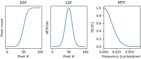
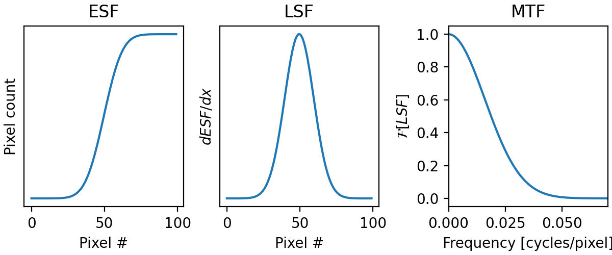
The Modulation Transfer Function (MTF) can be determined from an edge spread function (ESF) by first calculating the line spread function (LSF) from the ESF, then taking the Fourier transform of the LSF. The magnitude of the resulting complex function is the MTF.

(Source code, png, hires.png, pdf)

Implementation

In pylinac, the MTF is computed from a list of profiles (edge spread functions) for example, multiple profiles taken at different edge positions of a phantom. The profiles can have different lengths (by default they are padded to a common size). Since it is not guaranteed that all profiles are aligned, the MTF is calculated for each profile individually, and then the results are averaged to obtain a single MTF.

It is assumed that the sample spacing (input parameter in mm) is the same for all profiles.

• If sample_spacing is None (default) the frequency axis is expressed in cycles per sample, up to 0.5 (Nyquist frequency).

• If sample_spacing is provided, the frequency axis is expressed in line pairs per mm, up to the Nyquist limit determined by the sample spacing.

# Default: frequency axis is expressd in cycles/sample
EdgeSpreadFunctionMTF(...)
# Same as above
EdgeSpreadFunctionMTF(..., sample_spacing = None)
# Sample_spacing in mm: frequency axis is expressd in line pairs/mm
EdgeSpreadFunctionMTF(..., sample_spacing = 0.5)

Each profile MTF is computed using the following sequence of operations:

1. Differentiate ESF → LSF

   Compute the line spread function (LSF) as the discrete derivative of the ESF, implemented with a central-difference method (lsf = np.gradient(esf)).

2. Apply windowing

   Multiply the LSF by a windowing function to taper the edges and reduce spectral leakage introduced by the finite measurement length. The default window is scipy.signal.windows.hann. This can be modified using the windowing parameter. Input arguments to the windowing function can also be passed in the constructor through kwargs.

   (see more windowing functions here: https://docs.scipy.org/doc/scipy/reference/signal.windows.html)

   # Default window: Hann
   EdgeSpreadFunctionMTF(...)
   # No windowing
   EdgeSpreadFunctionMTF(..., windowing=None)
   # Custom window with default parameters
   EdgeSpreadFunctionMTF(..., windowing=scipy.signal.windows.tukey)
   # Custom window with custom parameters
   EdgeSpreadFunctionMTF(..., windowing=scipy.signal.windows.tukey, alpha=0.3)
   

3. Zero-pad for frequency resolution

   Pad the LSF to the target length (default: 1024 samples). Padding does not add information, but interpolates the frequency spectrum more finely, improving the resolution of the displayed MTF curve. This can be modified using the parameters padding_mode and num_samples:

   # no padding
   EdgeSpreadFunctionMTF(..., padding_mode="none")
   # array zero-padded to 2048 elements (must be larger than the largest array)
   EdgeSpreadFunctionMTF(..., padding_mode="fixed", num_samples=2048)
   # array padded to the next power of 2 or num_samples
   (i.e. len(largest_array) == 200 => num_samples=1024, len(largest_array) == 1025 => num_samples=2048)
   EdgeSpreadFunctionMTF(..., padding_mode="auto", num_samples=1024)
   

4. Fourier transform

   Compute the fast Fourier transform (FFT) of the windowed and padded LSF.

5. Magnitude spectrum → MTF

   Take the modulus (magnitude) of the FFT result to obtain the (unnormalized) MTF.

6. Normalization

   Normalize the MTF by dividing by the first value so that MTF(0) = 1.

Moments-based MTF

The MTF can also be calculated using the moments of the line pair spread function (LPSF). This algorithm is based on the work of Hander et al [1]. Specifically, equation 8:

\[MTF = \frac{\sqrt{2 * (\sigma^{2} - \mu)}}{\mu}\]

where \(\mu\) is the mean pixel value of the ROI and \(\sigma\) is the standard deviation of the ROI pixel values.

[1]

Hander et al. “Rapid objective measurement of gamma camera resolution using statistical moments” (1998).

API Documentation

class pylinac.core.mtf.MTF(lp_spacings: Sequence[float], lp_maximums: Sequence[float], lp_minimums: Sequence[float])

Bases: object

This class will calculate relative MTF

Parameters

lp_spacingssequence of floats

These are the physical spacings per unit distance. E.g. 0.1 line pairs/mm.

lp_maximumssequence of floats

These are the maximum values of the sample ROIs.

lp_minimumssequence of floats

These are the minimum values of the sample ROIs.

relative_resolution(x: float = 50) → float

Return the line pair value at the given rMTF resolution value.

Parameters

xfloat

The percentage of the rMTF to determine the line pair value. Must be between 0 and 100.

classmethod from_high_contrast_diskset(spacings: Sequence[float], diskset: Sequence[HighContrastDiskROI | RectangleROI]) → MTF

Construct the MTF using high contrast disks from the ROI module.

plotly(fig: Figure | None = None, x_label: str = 'Line pairs / mm', y_label: str = 'Relative MTF', title: str = 'Relative MTF', name: str = 'rMTF', **kwargs) → Figure

Plot the Relative MTF.

Parameters

plot(axis: Axes | None = None, grid: bool = True, x_label: str = 'Line pairs / mm', y_label: str = 'Relative MTF', title: str = 'RMTF', margins: float = 0.05, marker: str = 'o', label: str = 'rMTF') → list[Line2D]

Plot the Relative MTF.

Parameters

axisNone, matplotlib.Axes

The axis to plot the MTF on. If None, will create a new figure.

class pylinac.core.mtf.PeakValleyMTF(lp_spacings: Sequence[float], lp_maximums: Sequence[float], lp_minimums: Sequence[float])

Bases: MTF

Parameters

lp_spacingssequence of floats

These are the physical spacings per unit distance. E.g. 0.1 line pairs/mm.

lp_maximumssequence of floats

These are the maximum values of the sample ROIs.

lp_minimumssequence of floats

These are the minimum values of the sample ROIs.

pylinac.core.mtf.moments_mtf(mean: float, std: float) → float

The moments-based MTF based on Hander et al 1997 Equation 8.

See Also

https://aapm.onlinelibrary.wiley.com/doi/epdf/10.1118/1.597928

pylinac.core.mtf.moments_fwhm(width: float, mean: float, std: float) → float

The moments-based FWHM based on Hander et al 1997 Equation A8.

Parameters

widthfloat

The bar width in mm

meanfloat

The mean of the ROI.

stdfloat

The standard deviation of the ROI.

See Also

https://aapm.onlinelibrary.wiley.com/doi/epdf/10.1118/1.597928

class pylinac.core.mtf.MomentMTF(lpmms: Sequence[float], means: Sequence[float], stds: Sequence[float])

Bases: object

A moments-based MTF. Based on the work of Hander et al 1997.

Parameters

lpmmssequence of floats

The line pairs per mm.

meanssequence of floats

The means of the ROIs.

stdssequence of floats

The standard deviations of the ROIs.

See Also

https://aapm.onlinelibrary.wiley.com/doi/epdf/10.1118/1.597928

classmethod from_high_contrast_diskset(lpmms: Sequence[float], diskset: Sequence[HighContrastDiskROI]) → MomentMTF

Construct the MTF using high contrast disks from the ROI module.

plot(axis: Axes | None = None, marker: str = 'o') → Axes

Plot the Relative MTF.

Parameters

axisNone, matplotlib.Axes

The axis to plot the MTF on. If None, will create a new figure.

class pylinac.core.mtf.EdgeSpreadFunctionMTF(esf: list[~numpy.ndarray], sample_spacing: float | None = None, padding_mode: ~typing.Literal['none', 'fixed', 'auto'] = 'auto', num_samples: int = 1024, windowing: ~collections.abc.Callable | None = <function hann>, **kwargs: ~typing.Any)

Bases: object

This class will calculate relative MTF from multiple edge spread function (ESF) The MTF is calculated for each ESF and the output is the average of all.

Parameters

esflist[ndarray]

These are the edge spread functions (ESF). Each element of the list represents an ESF.

sample_spacingfloat | None

This is the sample spacing in mm. If None, the frequency axis is cycles/pixel, otherwise it’s converted to lp/mm. Default is None.

padding_modeLiteral[“none”, “fixed”, “auto”]

This is the padding mode (adding zeros) to increase resolution. Default is “auto”

• mode=”none”: array is unchanged

• mode=”fixed”: pad to num_samples (must be larger than the largest array)

• mode=”auto”: pad to the next power of two from the number of samples and num_samples

num_samplesint

This is the size of the array after padding. Only applicable if padding_mode is “fixed” or “auto”. Default is 1024

windowingCallable | None

This is the function used to window the ESF. Default is Hann window.

kwargs

These are the parameters to be used when calling windowing, ie windowing(kwargs)

relative_resolution(x: float = 50) → float

Return the line pair value at the given rMTF resolution value.

Parameters

xfloat

The percentage of the rMTF to determine the line pair value. Must be between 0 and 100.