“Cheese” Phantoms¶

Added in version 3.9.

Warning

These algorithms have only a limited amount of testing data and results should be scrutinized. Further, the algorithm is more likely to change in the future when a more robust test suite is built up. If you’d like to submit data, enter it here. Thanks!

The Cheese module provides routines for automatically analyzing DICOM images of phantoms commonly called “cheese” phantoms, defined by round phantoms with holes where the user can insert plugs, usually of known density. The primary use case is performing HU calibration or verification although some plugs allow for additional functionality such as spatial resolution. It can load a folder or zip file of images, correcting for translational and rotational offsets.

Phantoms Supported¶

The following phantoms are supported:

Tomotherapy Cheese TomoCheese
CIRS Electron Density CIRS062M

Image Acquisition¶

To be able to properly analyze the phantom, images should be acquired in such a way that the couch and phantom are separated. If the phantom it sitting in such a way that it is directly touching the couch analysis will likely fail. If the phantom does not come with a support device that keeps it off the table, it should be set on a low-density material such as foam blocks.

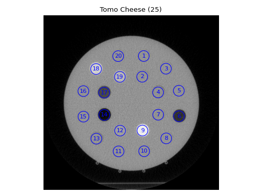
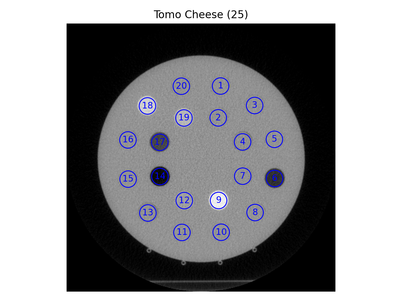
Running the Demo¶

To run one of the Cheese phantom demos, create a script or start an interpreter and input:

from pylinac import TomoCheese

TomoCheese.run_demo()

(Source code, png, hires.png, pdf)

Results will be also be printed to the console:

- TomoTherapy Cheese Phantom Analysis -
- HU Module -
ROI 1 median: 17.0, stdev: 37.9
ROI 2 median: 20.0, stdev: 44.2
ROI 3 median: 23.0, stdev: 36.9
ROI 4 median: 1.0, stdev: 45.7
ROI 5 median: 17.0, stdev: 37.6
ROI 6 median: -669.0, stdev: 39.6
ROI 7 median: 14.5, stdev: 45.8
ROI 8 median: 26.0, stdev: 38.6
ROI 9 median: 653.0, stdev: 47.4
ROI 10 median: 25.0, stdev: 36.7
ROI 11 median: 24.0, stdev: 35.3
ROI 12 median: 102.0, stdev: 46.2
ROI 13 median: 8.0, stdev: 38.1
ROI 14 median: -930.0, stdev: 43.8
ROI 15 median: 23.0, stdev: 36.3
ROI 16 median: 15.0, stdev: 37.1
ROI 17 median: -516.0, stdev: 45.1
ROI 18 median: 448.0, stdev: 38.1
ROI 19 median: 269.0, stdev: 45.3
ROI 20 median: 15.0, stdev: 37.9

Typical Use¶

The cheese phantom analyses follows a similar pattern of load/analyze/output as the rest of the library. Unlike the CatPhan analysis, tolerances are not applied and comparison to known values is not the goal. There are two reasons for this: 1) The plugs are interchangable and thus the reference values are not necessarily constant. 2) Evaluation against a reference is not the end goal as described in the philosophy. Thus, measured values are provided; what you do with them is your business.

To use the Tomo Cheese analysis, import the class:

from pylinac import TomoCheese

And then load, analyze, and view the results:

Load images – Loading can be done with a directory or zip file:

cheese_folder = r"C:/TomoTherapy/QA/September"
cheese = TomoCheese(cheese_folder)

or load from zip:

cheese_zip = r"C:/TomoTherapy/QA/September.zip"
cheese = TomoCheese.from_zip(cheese_zip)

Analyze – Analyze the dataset:
```
cheese.analyze()
```

View the results – Reviewing the results can be done in text or dictionary format as well as images:

# print text to the console
print(cheese.results())
# return a dictionary or dataclass
results = cheese.results_data()
# view analyzed image summary
cheese.plot_analyzed_image()
# save the images
cheese.save_analyzed_image()
# finally, save a PDF
cheese.publish_pdf()

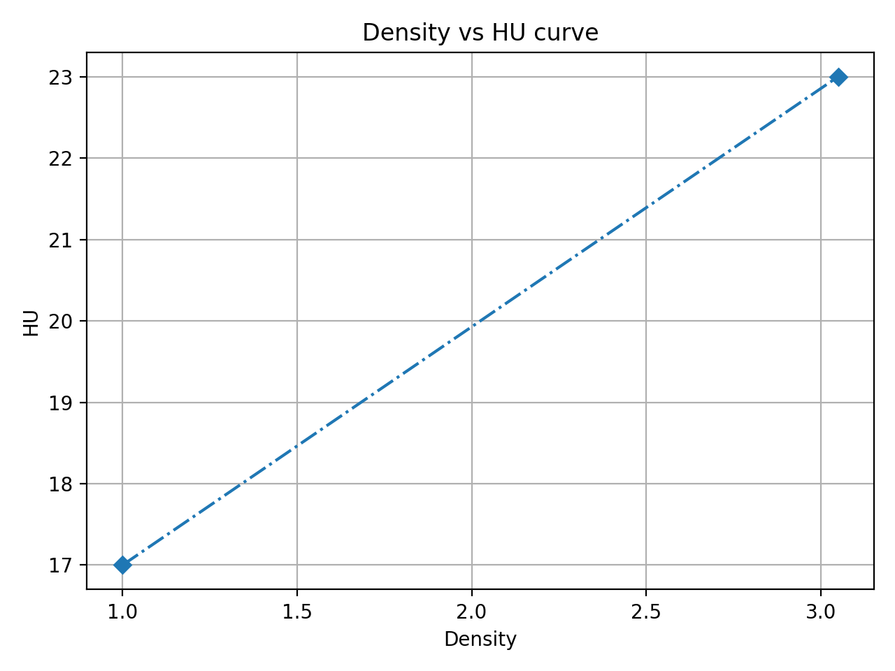
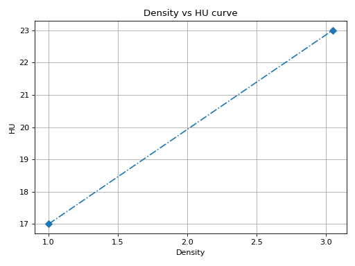
Plotting density¶

An HU-to-density curve can be plotted if an ROI configuration is passed to the analyze parameter like so:

import pylinac

density_info = {
    "1": {"density": 1.0},
    "3": {"density": 3.05},
}  # add more as needed. all keys must have a dict with 'density' defined
tomo = pylinac.TomoCheese(...)
tomo.analyze(roi_config=density_info)
tomo.plot_density_curve()  # in this case, ROI 1 and 3 will be plotted vs the stated density

This will plot a simple HU vs density graph.

(Source code, png, hires.png, pdf)

Note

The keys of the configuration must be strings matching the ROI number on the phantom. I.e. 1 matches to “ROI 1”, etc.

Note

Not all ROI densities have to be defined. Any ROI between 1 and 20 can be set.

Extending for other phantoms¶

While new commercial cheese-like phantoms will continue to be added to this module, creating new classes is relatively easy. The following steps show how this can be accomplished.

Create a new class “module” that inherits from CheeseModule. This class contains information about the ROIs, such as the distance and angle away from the center. You can use the TomoCheeseModule as a guide in the source code. An example:

from pylinac.cheese import CheeseModule


class SwissCheeseModule(CheeseModule):
    common_name = "Swiss cheese phantom"
    roi_settings = {  # configuration of each ROI.
        "1": {  # each ROI should have a string key and the following keys
            "angle": 90,
            "distance": 45,
            "radius": 6,
        },
        "2": {
            "angle": 45,
            "distance": 80,
            "radius": 6,
        },
        "3": {...},
    }

Note

Not all ROIs have to be defined. E.g. if you are only interested in 5 ROIs out of 20 then simply configure those 5.

Create a new class that inherits from CheesePhantomBase. This will define the phantom itself:

from pylinac.cheese import CheesePhantomBase


class SwissCheesePhantom(CheesePhantomBase):
    model = "Swiss Cheese Phantom"
    # generally this is just the radius of a normal ROI
    air_bubble_radius_mm = 14
    # This is the radius in mm to a "ring" of ROIs that is used for localization and roll determination.
    # Generally speaking, set the value to the ring that contains the highest ROI HUs.
    localization_radius = 110
    # minimum number of images that should be in the dataset
    min_num_images = 10
    # the radius of the phantom itself
    catphan_radius_mm = 150
    # set this to the module we just created above
    module_class = SwissModule
    # Optional: for the best type inference when using an IDE, set this as well to the new module. Note it's only a type annotation!!
    module: SwissModule

Use the class as normal. The base classes contain all the infrastructure code for analysis and plotting.
```
swiss = SwissCheesePhantom("my/swiss/data")
swiss.analyze()
swiss.plot_analyzed_image()
```

Algorithm¶

The TomoCheese algorithm leverages a lot of infrastructure from the CatPhan algorithm. It is not based on a manual.

Allowances¶

The images can be any size.
The phantom can have significant translation in all 3 directions.
The phantom can have significant roll and moderate yaw and pitch.

Restrictions¶

Warning

Analysis can fail or give unreliable results if any Restriction is violated.

The phantom cannot touch any edge of the FOV.
There must be at least one ROI in the “outer” ROI ring that is higher than water/background phantom. This has to do with the automatic roll compensation.

Note

This is not strictly required but will assist in accurate sub-degree roll compensation.

Pre-Analysis¶

The pre-analysis is almost exactly the same as the CatPhan pre-analysis.

Analysis¶

Determine image properties – Automatic roll compensation is attempted by creating a circular profile at the radius of the “outer” ROIs. This profile is then searched for peaks, which correspond to high-density plugs that have been inserted. If a peak is not found, no correction is applied and the phantom is assumed to be at 0. This would occur if all plugs have been filled with water/background plugs. If a peak is found, i.e. a plug has been inserted with HU detectably above water, the center of the peak is determined which would correspond to the center of the ROI. The distance to the nearest nominal ROI is calculated. If the value is <5 degrees, the roll compensation is applied. If the value is >5 degrees, the compensation is not applied and the phantom is assumed to be at 0.
Measure HU values of each plug – Based on the nominal spacing and roll compensation (if applied), each plug area is sampled for the median and standard deviation values.

API Documentation¶

class pylinac.cheese.TomoCheese(folderpath: str | Sequence[str] | Path | Sequence[Path] | Sequence[BytesIO], check_uid: bool = True, memory_efficient_mode: bool = False)[source]¶

Bases: CheesePhantomBase, ResultsDataMixin[TomoCheeseResult]

A class for analyzing the TomoTherapy ‘Cheese’ Phantom containing insert holes and plugs for HU analysis.

Parameters¶

folderpathstr, list of strings, or Path to folder: String that points to the CBCT image folder location.
check_uidbool: Whether to enforce raising an error if more than one UID is found in the dataset.
memory_efficient_modebool: Whether to use a memory efficient mode. If True, the DICOM stack will be loaded on demand rather than all at once. This will reduce the memory footprint but will be slower by ~25%. Default is False.

Raises¶

NotADirectoryError: If folder str passed is not a valid directory.
FileNotFoundError: If no CT images are found in the folder

module_class¶: alias of TomoCheeseModule

static run_demo(show: bool = True)[source]¶: Run the Tomotherapy Cheese demo

analyze(roi_config: dict | None = None) → None¶

Analyze the Tomo Cheese phantom.

Parameters¶

roi_configdict: The configuration of the ROIs, specifically the known densities.

property catphan_size: float¶: The expected size of the phantom in pixels, based on a 20cm wide phantom.

find_origin_slice() → int¶

Using a brute force search of the images, find the median HU linearity slice.

This method walks through all the images and takes a collapsed circle profile where the HU linearity ROIs are. If the profile contains both low (<800) and high (>800) HU values and most values are the same (i.e. it’s not an artifact), then it can be assumed it is an HU linearity slice. The median of all applicable slices is the center of the HU slice.

Returns¶

int: The middle slice of the HU linearity module.

find_phantom_axis()¶

We fit all the center locations of the phantom across all slices to a 1D poly function instead of finding them individually for robustness.

Normally, each slice would be evaluated individually, but the RadMachine jig gets in the way of detecting the HU module (🤦‍♂️). To work around that in a backwards-compatible way we instead look at all the slices and if the phantom was detected, capture the phantom center. ALL the centers are then fitted to a 1D poly function and passed to the individual slices. This way, even if one slice is messed up (such as because of the phantom jig), the poly function is robust to give the real center based on all the other properly-located positions on the other slices.

find_phantom_roll(func: Callable | None = None) → float¶: Examine the phantom for the maximum HU delta insert position. Roll the phantom by the measured angle to the nearest nominal angle if nearby. If not nearby, default to 0

classmethod from_demo_images()¶: Construct a CBCT object from the demo images.

classmethod from_url(url: str, check_uid: bool = True)¶

Instantiate a CBCT object from a URL pointing to a .zip object.

Parameters¶

urlstr: URL pointing to a zip archive of CBCT images.
check_uidbool: Whether to enforce raising an error if more than one UID is found in the dataset.

classmethod from_zip(zip_file: str | ZipFile | BinaryIO, check_uid: bool = True, memory_efficient_mode: bool = False)¶

Construct a CBCT object and pass the zip file.

Parameters¶

zip_filestr, ZipFile: Path to the zip file or a ZipFile object.
check_uidbool: Whether to enforce raising an error if more than one UID is found in the dataset.
memory_efficient_modebool: Whether to use a memory efficient mode. If True, the DICOM stack will be loaded on demand rather than all at once. This will reduce the memory footprint but will be slower by ~25%. Default is False.

Raises¶

FileExistsError : If zip_file passed was not a legitimate zip file. FileNotFoundError : If no CT images are found in the folder

localize() → None¶: Find the slice number of the catphan’s HU linearity module and roll angle

property mm_per_pixel: float¶: The millimeters per pixel of the DICOM images.

property num_images: int¶: The number of images loaded.

plot_analyzed_image(show: bool = True, **plt_kwargs: dict) → None¶

Plot the images used in the calculation and summary data.

Parameters¶

showbool: Whether to plot the image or not.
plt_kwargsdict: Keyword args passed to the plt.figure() method. Allows one to set things like figure size.

plot_analyzed_subimage() → None¶

Plot a specific component of the CBCT analysis.

Parameters¶

subimage{‘hu’, ‘un’, ‘sp’, ‘lc’, ‘mtf’, ‘lin’, ‘prof’, ‘side’}

The subcomponent to plot. Values must contain one of the following letter combinations. E.g. linearity, linear, and lin will all draw the HU linearity values.

hu draws the HU linearity image.
un draws the HU uniformity image.
sp draws the Spatial Resolution image.
lc draws the Low Contrast image (if applicable).
mtf draws the RMTF plot.
lin draws the HU linearity values. Used with delta.
prof draws the HU uniformity profiles.
side draws the side view of the phantom with lines of the module locations.

deltabool

Only for use with lin. Whether to plot the HU delta or actual values.

showbool

Whether to actually show the plot.

plot_density_curve(show: bool = True, **plt_kwargs: dict)¶

Plot the densities of the ROIs vs the measured HU. This will sort the ROIs by measured HU before plotting.

Parameters¶

showbool: Whether to plot the image or not.
plt_kwargsdict: Keyword args passed to the plt.figure() method. Allows one to set things like figure size.

plot_side_view(axis: Axes) → None¶: Plot a view of the scan from the side with lines showing detected module positions

Publish (print) a PDF containing the analysis and quantitative results.

Parameters¶

filename(str, file-like object}: The file to write the results to.
notesstr, list of strings: Text; if str, prints single line. If list of strings, each list item is printed on its own line.
open_filebool: Whether to open the file using the default program after creation.
metadatadict: Extra data to be passed and shown in the PDF. The key and value will be shown with a colon. E.g. passing {‘Author’: ‘James’, ‘Unit’: ‘TrueBeam’} would result in text in the PDF like: ————– Author: James Unit: TrueBeam ————–
logo: Path, str: A custom logo to use in the PDF report. If nothing is passed, the default pylinac logo is used.

refine_origin_slice(initial_slice_num: int) → int¶: Apply a refinement to the origin slice. This was added to handle the catphan 604 at least due to variations in the length of the HU plugs.

results(as_list: bool = False) → str | list[str]¶

Return the results of the analysis as a string. Use with print().

Parameters¶

as_listbool: Whether to return as a list of strings vs single string. Pretty much for internal usage.

results_data(as_dict: bool = False, as_json: bool = False) → T | dict | str¶

Present the results data and metadata as a dataclass, dict, or tuple. The default return type is a dataclass.

Parameters¶

as_dictbool: If True, return the results as a dictionary.
as_jsonbool: If True, return the results as a JSON string. Cannot be True if as_dict is True.

save_analyzed_image(filename: str | Path | BinaryIO, **kwargs) → None¶

Save the analyzed summary plot.

Parameters¶

filenamestr, file object: The name of the file to save the image to.
kwargs :: Any valid matplotlib kwargs.

save_analyzed_subimage() → None¶

Save a component image to file.

Parameters¶

filenamestr, file object: The file to write the image to.
subimagestr: See plot_analyzed_subimage() for parameter info.
deltabool: Only for use with lin. Whether to plot the HU delta or actual values.

class pylinac.cheese.CIRS062M(folderpath: str | Sequence[str] | Path | Sequence[Path] | Sequence[BytesIO], check_uid: bool = True, memory_efficient_mode: bool = False)[source]¶

Bases: CheesePhantomBase

A class for analyzing the CIRS Electron Density Phantom containing insert holes and plugs for HU analysis.

Parameters¶

folderpathstr, list of strings, or Path to folder: String that points to the CBCT image folder location.
check_uidbool: Whether to enforce raising an error if more than one UID is found in the dataset.
memory_efficient_modebool: Whether to use a memory efficient mode. If True, the DICOM stack will be loaded on demand rather than all at once. This will reduce the memory footprint but will be slower by ~25%. Default is False.

Raises¶

NotADirectoryError: If folder str passed is not a valid directory.
FileNotFoundError: If no CT images are found in the folder

module_class¶: alias of CIRSHUModule

classmethod from_demo_images()[source]¶: Construct a CBCT object from the demo images.

find_origin_slice() → int[source]¶: We override to lower the minimum variation required. This is ripe for refactor, but I’d like to add a few more phantoms first to get the full picture required.

analyze(roi_config: dict | None = None) → None¶

Analyze the Tomo Cheese phantom.

Parameters¶

roi_configdict: The configuration of the ROIs, specifically the known densities.

property catphan_size: float¶: The expected size of the phantom in pixels, based on a 20cm wide phantom.

find_phantom_axis()¶

We fit all the center locations of the phantom across all slices to a 1D poly function instead of finding them individually for robustness.

find_phantom_roll(func: Callable | None = None) → float¶: Examine the phantom for the maximum HU delta insert position. Roll the phantom by the measured angle to the nearest nominal angle if nearby. If not nearby, default to 0

classmethod from_url(url: str, check_uid: bool = True)¶

Instantiate a CBCT object from a URL pointing to a .zip object.

Parameters¶

urlstr: URL pointing to a zip archive of CBCT images.
check_uidbool: Whether to enforce raising an error if more than one UID is found in the dataset.

classmethod from_zip(zip_file: str | ZipFile | BinaryIO, check_uid: bool = True, memory_efficient_mode: bool = False)¶

Construct a CBCT object and pass the zip file.

Parameters¶

zip_filestr, ZipFile: Path to the zip file or a ZipFile object.
check_uidbool: Whether to enforce raising an error if more than one UID is found in the dataset.
memory_efficient_modebool: Whether to use a memory efficient mode. If True, the DICOM stack will be loaded on demand rather than all at once. This will reduce the memory footprint but will be slower by ~25%. Default is False.

Raises¶

FileExistsError : If zip_file passed was not a legitimate zip file. FileNotFoundError : If no CT images are found in the folder

localize() → None¶: Find the slice number of the catphan’s HU linearity module and roll angle

property mm_per_pixel: float¶: The millimeters per pixel of the DICOM images.

property num_images: int¶: The number of images loaded.

plot_analyzed_image(show: bool = True, **plt_kwargs: dict) → None¶

Plot the images used in the calculation and summary data.

Parameters¶

showbool: Whether to plot the image or not.
plt_kwargsdict: Keyword args passed to the plt.figure() method. Allows one to set things like figure size.

plot_analyzed_subimage() → None¶

Plot a specific component of the CBCT analysis.

Parameters¶

subimage{‘hu’, ‘un’, ‘sp’, ‘lc’, ‘mtf’, ‘lin’, ‘prof’, ‘side’}

The subcomponent to plot. Values must contain one of the following letter combinations. E.g. linearity, linear, and lin will all draw the HU linearity values.

hu draws the HU linearity image.
un draws the HU uniformity image.
sp draws the Spatial Resolution image.
lc draws the Low Contrast image (if applicable).
mtf draws the RMTF plot.
lin draws the HU linearity values. Used with delta.
prof draws the HU uniformity profiles.
side draws the side view of the phantom with lines of the module locations.

deltabool

Only for use with lin. Whether to plot the HU delta or actual values.

showbool

Whether to actually show the plot.

plot_density_curve(show: bool = True, **plt_kwargs: dict)¶

Plot the densities of the ROIs vs the measured HU. This will sort the ROIs by measured HU before plotting.

Parameters¶

showbool: Whether to plot the image or not.
plt_kwargsdict: Keyword args passed to the plt.figure() method. Allows one to set things like figure size.

plot_side_view(axis: Axes) → None¶: Plot a view of the scan from the side with lines showing detected module positions

Publish (print) a PDF containing the analysis and quantitative results.

Parameters¶

filename(str, file-like object}: The file to write the results to.
notesstr, list of strings: Text; if str, prints single line. If list of strings, each list item is printed on its own line.
open_filebool: Whether to open the file using the default program after creation.
metadatadict: Extra data to be passed and shown in the PDF. The key and value will be shown with a colon. E.g. passing {‘Author’: ‘James’, ‘Unit’: ‘TrueBeam’} would result in text in the PDF like: ————– Author: James Unit: TrueBeam ————–
logo: Path, str: A custom logo to use in the PDF report. If nothing is passed, the default pylinac logo is used.

refine_origin_slice(initial_slice_num: int) → int¶: Apply a refinement to the origin slice. This was added to handle the catphan 604 at least due to variations in the length of the HU plugs.

results(as_list: bool = False) → str | list[str]¶

Return the results of the analysis as a string. Use with print().

Parameters¶

as_listbool: Whether to return as a list of strings vs single string. Pretty much for internal usage.

results_data(as_dict: bool = False, as_json: bool = False) → T | dict | str¶

Present the results data and metadata as a dataclass, dict, or tuple. The default return type is a dataclass.

Parameters¶

as_dictbool: If True, return the results as a dictionary.
as_jsonbool: If True, return the results as a JSON string. Cannot be True if as_dict is True.

save_analyzed_image(filename: str | Path | BinaryIO, **kwargs) → None¶

Save the analyzed summary plot.

Parameters¶

filenamestr, file object: The name of the file to save the image to.
kwargs :: Any valid matplotlib kwargs.

save_analyzed_subimage() → None¶

Save a component image to file.

Parameters¶

filenamestr, file object: The file to write the image to.
subimagestr: See plot_analyzed_subimage() for parameter info.
deltabool: Only for use with lin. Whether to plot the HU delta or actual values.

class pylinac.cheese.TomoCheeseModule(catphan, tolerance: float | None = None, offset: int = 0, clear_borders: bool = True)[source]¶

Bases: CheeseModule

The pluggable module with user-accessible holes.

The ROIs of the inner circle are ~45 degrees apart. The ROIs of the outer circle are ~30 degrees apart.

Parameters¶

catphanCatPhanBase instance.: The catphan instance.
slice_numint: The slice number of the DICOM array desired. If None, will use the slice_num property of subclass.
combinebool: If True, combines the slices +/- num_slices around the slice of interest to improve signal/noise.
combine_method{‘mean’, ‘max’}: How to combine the slices if combine is True.
num_slicesint: The number of slices on either side of the nominal slice to combine to improve signal/noise; only applicable if combine is True.
clear_bordersbool: If True, clears the borders of the image to remove any ROIs that may be present.
original_imageImage or None: The array of the slice. This is a bolt-on parameter for optimization. Leaving as None is fine, but can increase analysis speed if 1) this image is passed and 2) there is no combination of slices happening, which is most of the time.

is_phantom_in_view() → bool¶: Whether the phantom appears to be within the slice.

property phan_center: Point¶: Determine the location of the center of the phantom.

property phantom_roi: RegionProperties¶

Get the Scikit-Image ROI of the phantom

The image is analyzed to see if: 1) the CatPhan is even in the image (if there were any ROIs detected) 2) an ROI is within the size criteria of the catphan 3) the ROI area that is filled compared to the bounding box area is close to that of a circle

plot(axis: Axes)¶: Plot the image along with ROIs to an axis

plot_rois(axis: Axes) → None¶: Plot the ROIs to the axis. We add the ROI # to help the user differentiate

preprocess(catphan)¶: A preprocessing step before analyzing the CTP module.

Parameters¶

catphan : ~pylinac.cbct.CatPhanBase instance.

roi_dist_mm¶: alias of float

property slice_num: int¶: The slice number of the spatial resolution module.

Returns¶

float

class pylinac.cheese.CIRSHUModule(catphan, tolerance: float | None = None, offset: int = 0, clear_borders: bool = True)[source]¶

Bases: CheeseModule

The pluggable module with user-accessible holes.

The ROIs of each circle are ~45 degrees apart.

Parameters¶

catphanCatPhanBase instance.: The catphan instance.
slice_numint: The slice number of the DICOM array desired. If None, will use the slice_num property of subclass.
combinebool: If True, combines the slices +/- num_slices around the slice of interest to improve signal/noise.
combine_method{‘mean’, ‘max’}: How to combine the slices if combine is True.
num_slicesint: The number of slices on either side of the nominal slice to combine to improve signal/noise; only applicable if combine is True.
clear_bordersbool: If True, clears the borders of the image to remove any ROIs that may be present.
original_imageImage or None: The array of the slice. This is a bolt-on parameter for optimization. Leaving as None is fine, but can increase analysis speed if 1) this image is passed and 2) there is no combination of slices happening, which is most of the time.

is_phantom_in_view() → bool¶: Whether the phantom appears to be within the slice.

property phan_center: Point¶: Determine the location of the center of the phantom.

property phantom_roi: RegionProperties¶

Get the Scikit-Image ROI of the phantom

plot(axis: Axes)¶: Plot the image along with ROIs to an axis

plot_rois(axis: Axes) → None¶: Plot the ROIs to the axis. We add the ROI # to help the user differentiate

preprocess(catphan)¶: A preprocessing step before analyzing the CTP module.

Parameters¶

catphan : ~pylinac.cbct.CatPhanBase instance.

roi_dist_mm¶: alias of float

property slice_num: int¶: The slice number of the spatial resolution module.

Returns¶

float

class pylinac.cheese.CheeseResult(*, pylinac_version: str = '3.22.0', date_of_analysis: datetime = None, origin_slice: int, num_images: int, phantom_roll: float, rois: dict)[source]¶

Bases: ResultBase

This class should not be called directly. It is returned by the results_data() method. It is a dataclass under the hood and thus comes with all the dunder magic.

Use the following attributes as normal class attributes.

Create a new model by parsing and validating input data from keyword arguments.

Raises [ValidationError][pydantic_core.ValidationError] if the input data cannot be validated to form a valid model.

self is explicitly positional-only to allow self as a field name.

origin_slice: int¶

num_images: int¶

phantom_roll: float¶

rois: dict¶

model_computed_fields: ClassVar[dict[str, ComputedFieldInfo]] = {}¶: A dictionary of computed field names and their corresponding ComputedFieldInfo objects.

model_config: ClassVar[ConfigDict] = {'arbitrary_types_allowed': True}¶: Configuration for the model, should be a dictionary conforming to [ConfigDict][pydantic.config.ConfigDict].

Metadata about the fields defined on the model, mapping of field names to [FieldInfo][pydantic.fields.FieldInfo].

This replaces Model.__fields__ from Pydantic V1.

class pylinac.cheese.TomoCheeseResult(*, pylinac_version: str = '3.22.0', date_of_analysis: datetime = None, origin_slice: int, num_images: int, phantom_roll: float, rois: dict, roi_1: dict, roi_2: dict, roi_3: dict, roi_4: dict, roi_5: dict, roi_6: dict, roi_7: dict, roi_8: dict, roi_9: dict, roi_10: dict, roi_11: dict, roi_12: dict, roi_13: dict, roi_14: dict, roi_15: dict, roi_16: dict, roi_17: dict, roi_18: dict, roi_19: dict, roi_20: dict)[source]¶

Bases: ResultBase

This class should not be called directly. It is returned by the results_data() method. It is a dataclass under the hood and thus comes with all the dunder magic.

Use the following attributes as normal class attributes.

Create a new model by parsing and validating input data from keyword arguments.

Raises [ValidationError][pydantic_core.ValidationError] if the input data cannot be validated to form a valid model.

self is explicitly positional-only to allow self as a field name.

origin_slice: int¶

num_images: int¶

phantom_roll: float¶

rois: dict¶

roi_1: dict¶

roi_2: dict¶

roi_3: dict¶

roi_4: dict¶

roi_5: dict¶

roi_6: dict¶

roi_7: dict¶

roi_8: dict¶

roi_9: dict¶

roi_10: dict¶

roi_11: dict¶

roi_12: dict¶

roi_13: dict¶

roi_14: dict¶

roi_15: dict¶

roi_16: dict¶

roi_17: dict¶

roi_18: dict¶

roi_19: dict¶

roi_20: dict¶

model_computed_fields: ClassVar[dict[str, ComputedFieldInfo]] = {}¶: A dictionary of computed field names and their corresponding ComputedFieldInfo objects.

model_config: ClassVar[ConfigDict] = {'arbitrary_types_allowed': True}¶: Configuration for the model, should be a dictionary conforming to [ConfigDict][pydantic.config.ConfigDict].

model_fields: ClassVar[dict[str, FieldInfo]] = {'date_of_analysis': FieldInfo(annotation=datetime, required=False, default_factory=builtin_function_or_method), 'num_images': FieldInfo(annotation=int, required=True), 'origin_slice': FieldInfo(annotation=int, required=True), 'phantom_roll': FieldInfo(annotation=float, required=True), 'pylinac_version': FieldInfo(annotation=str, required=False, default='3.22.0'), 'roi_1': FieldInfo(annotation=dict, required=True), 'roi_10': FieldInfo(annotation=dict, required=True), 'roi_11': FieldInfo(annotation=dict, required=True), 'roi_12': FieldInfo(annotation=dict, required=True), 'roi_13': FieldInfo(annotation=dict, required=True), 'roi_14': FieldInfo(annotation=dict, required=True), 'roi_15': FieldInfo(annotation=dict, required=True), 'roi_16': FieldInfo(annotation=dict, required=True), 'roi_17': FieldInfo(annotation=dict, required=True), 'roi_18': FieldInfo(annotation=dict, required=True), 'roi_19': FieldInfo(annotation=dict, required=True), 'roi_2': FieldInfo(annotation=dict, required=True), 'roi_20': FieldInfo(annotation=dict, required=True), 'roi_3': FieldInfo(annotation=dict, required=True), 'roi_4': FieldInfo(annotation=dict, required=True), 'roi_5': FieldInfo(annotation=dict, required=True), 'roi_6': FieldInfo(annotation=dict, required=True), 'roi_7': FieldInfo(annotation=dict, required=True), 'roi_8': FieldInfo(annotation=dict, required=True), 'roi_9': FieldInfo(annotation=dict, required=True), 'rois': FieldInfo(annotation=dict, required=True)}¶

Metadata about the fields defined on the model, mapping of field names to [FieldInfo][pydantic.fields.FieldInfo].

This replaces Model.__fields__ from Pydantic V1.

class pylinac.cheese.CheesePhantomBase(folderpath: str | Sequence[str] | Path | Sequence[Path] | Sequence[BytesIO], check_uid: bool = True, memory_efficient_mode: bool = False)[source]¶

Bases: CatPhanBase, ResultsDataMixin[CheeseResult]

A base class for doing cheese-like phantom analysis. A subset of catphan analysis where only one module is assumed.

Parameters¶

folderpathstr, list of strings, or Path to folder: String that points to the CBCT image folder location.
check_uidbool: Whether to enforce raising an error if more than one UID is found in the dataset.
memory_efficient_modebool: Whether to use a memory efficient mode. If True, the DICOM stack will be loaded on demand rather than all at once. This will reduce the memory footprint but will be slower by ~25%. Default is False.

Raises¶

NotADirectoryError: If folder str passed is not a valid directory.
FileNotFoundError: If no CT images are found in the folder

analyze(roi_config: dict | None = None) → None[source]¶

Analyze the Tomo Cheese phantom.

Parameters¶

roi_configdict: The configuration of the ROIs, specifically the known densities.

find_phantom_roll(func: Callable | None = None) → float[source]¶: Examine the phantom for the maximum HU delta insert position. Roll the phantom by the measured angle to the nearest nominal angle if nearby. If not nearby, default to 0

plot_analyzed_image(show: bool = True, **plt_kwargs: dict) → None[source]¶

Plot the images used in the calculation and summary data.

Parameters¶

showbool: Whether to plot the image or not.
plt_kwargsdict: Keyword args passed to the plt.figure() method. Allows one to set things like figure size.

results(as_list: bool = False) → str | list[str][source]¶

Return the results of the analysis as a string. Use with print().

Parameters¶

as_listbool: Whether to return as a list of strings vs single string. Pretty much for internal usage.

plot_density_curve(show: bool = True, **plt_kwargs: dict)[source]¶

Plot the densities of the ROIs vs the measured HU. This will sort the ROIs by measured HU before plotting.

Parameters¶

showbool: Whether to plot the image or not.
plt_kwargsdict: Keyword args passed to the plt.figure() method. Allows one to set things like figure size.

Publish (print) a PDF containing the analysis and quantitative results.

Parameters¶

filename(str, file-like object}: The file to write the results to.
notesstr, list of strings: Text; if str, prints single line. If list of strings, each list item is printed on its own line.
open_filebool: Whether to open the file using the default program after creation.
metadatadict: Extra data to be passed and shown in the PDF. The key and value will be shown with a colon. E.g. passing {‘Author’: ‘James’, ‘Unit’: ‘TrueBeam’} would result in text in the PDF like: ————– Author: James Unit: TrueBeam ————–
logo: Path, str: A custom logo to use in the PDF report. If nothing is passed, the default pylinac logo is used.

save_analyzed_subimage() → None[source]¶

Save a component image to file.

Parameters¶

filenamestr, file object: The file to write the image to.
subimagestr: See plot_analyzed_subimage() for parameter info.
deltabool: Only for use with lin. Whether to plot the HU delta or actual values.

plot_analyzed_subimage() → None[source]¶

Plot a specific component of the CBCT analysis.

Parameters¶

subimage{‘hu’, ‘un’, ‘sp’, ‘lc’, ‘mtf’, ‘lin’, ‘prof’, ‘side’}

The subcomponent to plot. Values must contain one of the following letter combinations. E.g. linearity, linear, and lin will all draw the HU linearity values.

hu draws the HU linearity image.
un draws the HU uniformity image.
sp draws the Spatial Resolution image.
lc draws the Low Contrast image (if applicable).
mtf draws the RMTF plot.
lin draws the HU linearity values. Used with delta.
prof draws the HU uniformity profiles.
side draws the side view of the phantom with lines of the module locations.

deltabool

Only for use with lin. Whether to plot the HU delta or actual values.

showbool

Whether to actually show the plot.

property catphan_size: float¶: The expected size of the phantom in pixels, based on a 20cm wide phantom.

find_origin_slice() → int¶

Using a brute force search of the images, find the median HU linearity slice.

Returns¶

int: The middle slice of the HU linearity module.

find_phantom_axis()¶

We fit all the center locations of the phantom across all slices to a 1D poly function instead of finding them individually for robustness.

classmethod from_demo_images()¶: Construct a CBCT object from the demo images.

classmethod from_url(url: str, check_uid: bool = True)¶

Instantiate a CBCT object from a URL pointing to a .zip object.

Parameters¶

urlstr: URL pointing to a zip archive of CBCT images.
check_uidbool: Whether to enforce raising an error if more than one UID is found in the dataset.

classmethod from_zip(zip_file: str | ZipFile | BinaryIO, check_uid: bool = True, memory_efficient_mode: bool = False)¶

Construct a CBCT object and pass the zip file.

Parameters¶

zip_filestr, ZipFile: Path to the zip file or a ZipFile object.
check_uidbool: Whether to enforce raising an error if more than one UID is found in the dataset.
memory_efficient_modebool: Whether to use a memory efficient mode. If True, the DICOM stack will be loaded on demand rather than all at once. This will reduce the memory footprint but will be slower by ~25%. Default is False.

Raises¶

FileExistsError : If zip_file passed was not a legitimate zip file. FileNotFoundError : If no CT images are found in the folder

localize() → None¶: Find the slice number of the catphan’s HU linearity module and roll angle

property mm_per_pixel: float¶: The millimeters per pixel of the DICOM images.

property num_images: int¶: The number of images loaded.

plot_side_view(axis: Axes) → None¶: Plot a view of the scan from the side with lines showing detected module positions

refine_origin_slice(initial_slice_num: int) → int¶: Apply a refinement to the origin slice. This was added to handle the catphan 604 at least due to variations in the length of the HU plugs.

results_data(as_dict: bool = False, as_json: bool = False) → T | dict | str¶

Present the results data and metadata as a dataclass, dict, or tuple. The default return type is a dataclass.

Parameters¶

as_dictbool: If True, return the results as a dictionary.
as_jsonbool: If True, return the results as a JSON string. Cannot be True if as_dict is True.

save_analyzed_image(filename: str | Path | BinaryIO, **kwargs) → None¶

Save the analyzed summary plot.

Parameters¶

filenamestr, file object: The name of the file to save the image to.
kwargs :: Any valid matplotlib kwargs.

“Cheese” Phantoms¶

Phantoms Supported¶

Image Acquisition¶

Running the Demo¶

Typical Use¶

Plotting density¶

Extending for other phantoms¶

Algorithm¶

Allowances¶

Restrictions¶

Pre-Analysis¶

Analysis¶

API Documentation¶

Parameters¶

Raises¶

Parameters¶

Returns¶

Parameters¶

Parameters¶

Raises¶

Parameters¶

Parameters¶

Parameters¶

Parameters¶

Parameters¶

Parameters¶

Parameters¶

Parameters¶

See Also¶

Parameters¶

Raises¶

Parameters¶

Parameters¶

Parameters¶

Raises¶

Parameters¶

Parameters¶

Parameters¶

Parameters¶

Parameters¶

Parameters¶

Parameters¶

Parameters¶

Parameters¶

Parameters¶

Returns¶

Parameters¶

Parameters¶

Returns¶

Parameters¶

Raises¶

Parameters¶

Parameters¶

Parameters¶

Parameters¶

Parameters¶

Parameters¶

Parameters¶

Returns¶

Parameters¶

Parameters¶

Raises¶

Parameters¶

Parameters¶