Profiles & 1D Metrics¶

Profiles, in the context of pylinac, are 1D arrays of data that contain a single radiation field. Colloquially, these are what physicists might call an “inplane profile” or “crossplane profile” although the usage here is not restricted to those orientations.

Use Cases¶

Typical use cases for profiles are:

Calculating a metric such as flatness, symmetry, penumbra, etc.
Finding the center of the field.
Finding the field edges.

Assumptions & Constraints¶

There is one single, large radiation field in the profile.
The radiation field should not be at the edge of the array.
The radiation field should have a higher pixel value than the background. I.e. it should not be inverted.
The field does not have to be normalized, but generally it should be. Plugins may assume normalized data.
The field can be “horned” (i.e. have a dip in the middle) and/or contain a peak from an FFF field.
The field can be off-center, but the penumbra should be fully contained in the array.
The field can be skewed (e.g. a wedge field).
The field can have any resolution or no resolution.

Basic Usage¶

Out of the box, the profile classes can be used to find the center of the field, field width, and the field edges.

from pylinac.core.profile import FWXMProfile

profile = FWXMProfile(..., fwxm_height=50)
print(profile.center_idx)  # print the center of the field position
print(profile.field_edge_idx(side="left"))  # print the left field edge position
print(profile.field_width_px)  # print the field width in pixels
profile.plot()  # plot the profile

However, the real power of the profile classes is in the plugins that can be used to calculate custom metrics. See the plugins section for more information.

Legacy vs New Classes¶

The legacy class for analyzing profiles is SingleProfile. This class is frozen and will not receive updates.

The modern classes for analyzing profiles are FWXMProfile, InflectionDerivativeProfile, HillProfile. These classes deal with arrays only.

For physical profiles, i.e. something where the values have a physical size or location like an EPID profile or water tank scan, use the following classes: FWXMProfilePhysical, InflectionDerivativeProfilePhysical, HillProfilePhysical.

Important

You will almost always want the ...Physical variants of the classes as most profiles are from physical sources. Furthermore, some plugins will not work with the non-physical classes.

The difference between SingleProfile and the other classes is that SingleProfile is a swiss army knife. It can do almost everything the other classes can do and considerably more. However, the other classes are more specialized and thus more robust as well as a lot clearer and focused. Internally, pylinac uses the new specialized classes. The new classes also allow for plugins to be written and used much easier than with SingleProfile.

The SingleProfile class is more complicated to both read and use than the specialized classes. It’s also harder to test and maintain. Thus, the specialized classes have come about as a response.

What class to use¶

Note

Throughout the documentation examples, the FWXM variety is used, but all examples can be replaced with the other variants.

The following list is a guide to what class to use:

PDDs, TPRs, and similar depth-focused scans:
- Use any of the classes.
FWXMProfile/FWXMProfilePhysical
- Use when the beam is “flat”; no FFF beams.
- Can handle somewhat noisy data.
- Robust to background noise and asymmetric background data.
InflectionDerivativeProfile/InflectionDerivativeProfilePhysical:
- Use either when the beam is flat or peaked.
- Is not robust to salt and pepper noise or gently-sloping data.
- The profile should have relatively sharp slopes compared to the background and central region.
- This is a good default ceteris parabus.
HillProfile/HillProfilePhysical:
- Use either when the beam is flat or peaked.
- It is robust to salt and pepper noise.
- Do not use with sparse data such as IC profiler or similar where little data exists in the penumbra region.

Metric Plugins¶

The new profile classes discussed above allow for plugins to be written that can calculate metrics of the profile. For example, a penumbra plugin could be written that calculates the penumbra of the profile.

Several plugins are provided out of the box, and writing new plugins is straightforward.

Metrics are calculated by passing it as a list to the calculate method. The examples below show its usage.

Built-in Plugins¶

The following plugins are available out of the box:

Penumbra Right¶

PenumbraRightMetric This plugin calculates the right penumbra of the profile. The upper and lower bounds can be passed in as arguments. The default is 80/20.

Example usage:

profile = FWXMProfile(...)
profile.compute(metrics=[PenumbraRightMetric(upper=80, lower=20)])

Note

When using Inflection derivative or Hill profiles, the penumbra is based on the height of the edge, not the maximum value of the profile. E.g. assume an FFF profile normalized to 1.0 and penumbra bounds of 80/20. The penumbra will not be at 50% height for Inflection derivative or Hill profiles. If it is detected at 0.4, or 40% height, the lower penumbra will be set to 20% (0.2) * 2 * 0.4, or 0.16. The upper penumbra will be 80% (0.8) * 2 * 0.4, or 0.64. This is because the penumbra bound is based on the height of the field edge, not the maximum value of the profile. 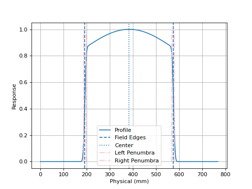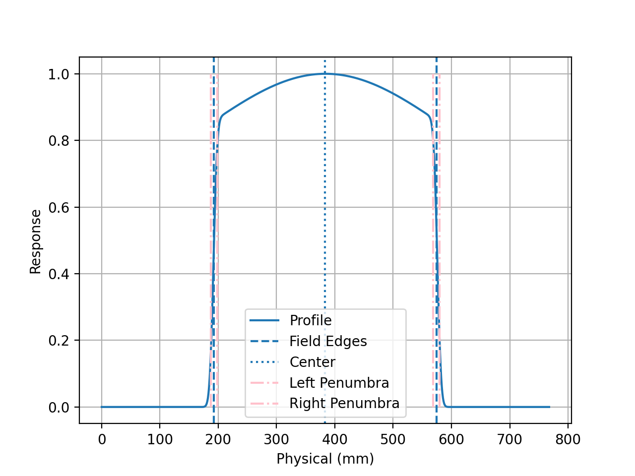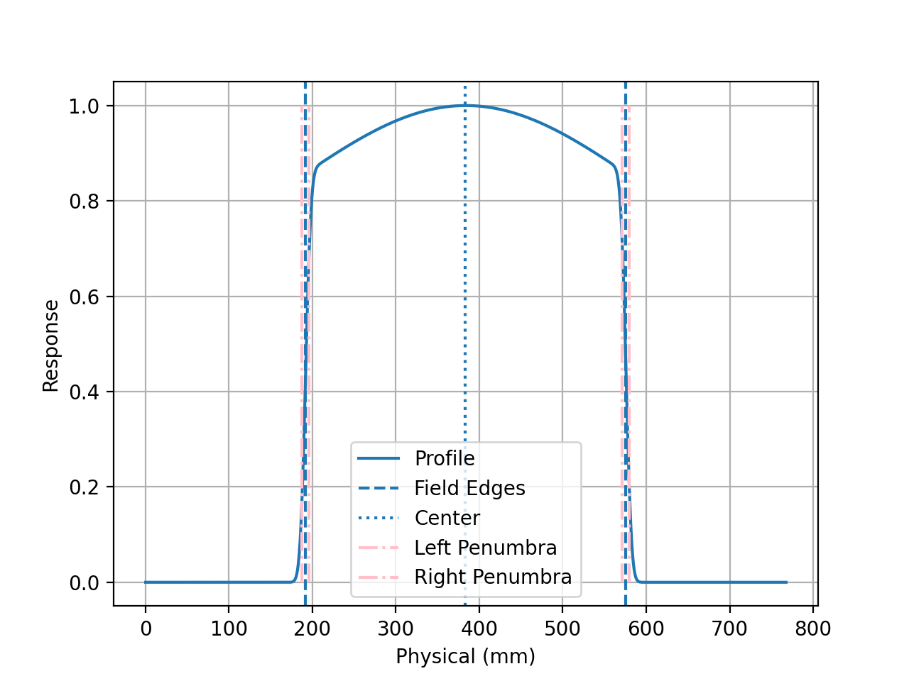This is best illustrated with a plot. We use the FWXMProfilePhysical class first to show its inappropriate use with FFF beams:

(Source code, png, hires.png, pdf)

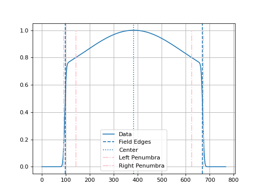
Note the upper penumbra is well-past the “shoulder” region and thus the penumbra is not accurate. Now let’s use the InflectionDerivativeProfilePhysical class:

(Source code, png, hires.png, pdf)

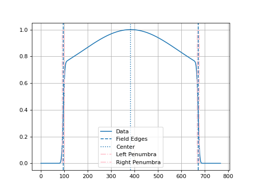
When analyzing flat beams, the FWXMProfile class is appropriate and will give similar results to the other two classes.

Penumbra Left¶

PenumbraLeftMetric This plugin calculates the left penumbra of the profile. The upper and lower bounds can be passed in as arguments. The default is 80/20.

Flatness (Difference)¶

FlatnessDifferenceMetric This plugin calculates the flatness difference of the profile. The in-field ratio can be passed in as an argument. The default is 0.8.

The flatness equation is:

\[flatness = 100 * \frac{D_{max} - D_{min}}{D_{max} + D_{min}} \in field\]

The equation does not track which side the flatness is higher or lower on. The value can range from 0 to 100. A perfect value is 0.

Example usage:

profile = FWXMProfile(...)
profile.compute(metrics=[FlatnessDifferenceMetric(in_field_ratio=0.8)])

Flatness (Ratio)¶

FlatnessRatioMetric This plugin calculates the flatness ratio of the profile. The in-field ratio can be passed in as an argument. The default is 0.8.

The flatness equation is:

\[flatness = 100 * \frac{D_{max}}{D_{min}} \in field\]

The equation does not track which side the flatness is higher or lower on. The value will range from 100 to \(\infty\). A perfect value is 100.

Example usage:

profile = FWXMProfile(...)
profile.compute(metrics=[FlatnessRatioMetric(in_field_ratio=0.8)])

Symmetry (Point Difference)¶

SymmetryPointDifferenceMetric This plugin calculates the symmetry point difference of the profile. The in-field ratio can be passed in as an argument. The default is 0.8.

The symmetry point difference equation is:

\[symmetry = 100 * \frac{max(L_{pt} - R_{pt})}{D_{CAX}} \in field\]

where \(L_{pt}\) and \(R_{pt}\) are equidistant from the beam center. Symmetry can be positive or negative. The \(max\) refers to the point with the maximum difference between the left and right points. If the largest absolute value is negative, that is the value used.

Note

Unlike the point difference quotient, this metric is signed. A negative value means the right side is higher. A positive value means the left side is higher.

Example usage:

profile = FWXMProfile(...)
profile.compute(metrics=[SymmetryPointDifferenceMetric(in_field_ratio=0.8)])

Symmetry (Point Difference Quotient)¶

SymmetryPointDifferenceQuotientMetric This plugin calculates the symmetry point difference of the profile defined as the Point Difference Quotient (aka IEC). The in-field ratio can be passed in as an argument. The default is 0.8.

The symmetry point difference equation is:

\[symmetry = 100 * max(\frac{L_{pt}}{R_{pt}}, \frac{R_{pt}}{L_{pt}}) \in field\]

where \(L_{pt}\) and \(R_{pt}\) are equidistant from the beam center. This value can range from 100 to \(\infty\). A perfect value is 100.

Example usage:

profile = FWXMProfile(...)
profile.compute(metrics=[SymmetryPointDifferenceQuotientMetric(in_field_ratio=0.8)])

Symmetry (Area)¶

SymmetryAreaMetric This plugin calculates the symmetry area of the profile. The in-field ratio can be passed in as an argument. The default is 0.8.

The symmetry area equation is:

\[symmetry = 100 * \frac{area_{left} - area_{right}}{area_{left} + area_{right}} \in field\]

where \(area_{left}\) and \(area_{right}\) are the areas under the left and right sides of the profile, centered about the beam center.

The value is signed. A negative value means the right side is higher and vice versa. The value can range from \(-100\) to \(+100\). A perfect value is 0.

Example usage:

profile = FWXMProfile(...)
profile.compute(metrics=[SymmetryAreaMetric(in_field_ratio=0.8)])

Top Position¶

TopPositionMetric This plugin calculates the distance from the “top” of the field to the beam center. This is typically used for FFF beams.

The calculation is based on the NCS-33 report. The central part of the field, by default the central 20%, is fitted to a 2nd order polynomial. The maximum of the polynomial is the “top” and the distance to the field center is calculated.

Example usage:

profile = FWXMProfile(...)
profile.compute(metrics=[TopDistanceMetric(top_region_ratio=0.2)])

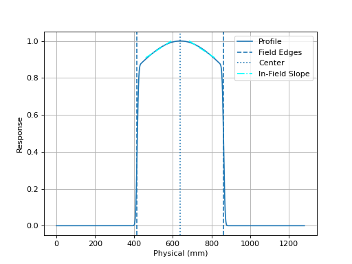
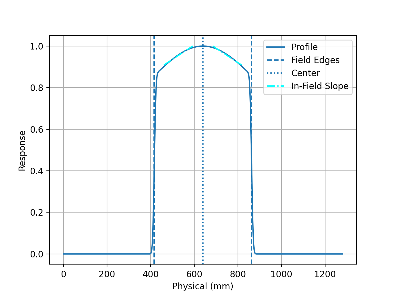
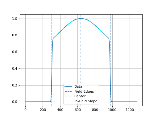
Field Slope¶

NCS-33 defined a field slope metric that used “Profile evaluation points” at various distances from the CAX. These points were averaged from the left and right sides and used as constancy values. Pylinac does something similar with the SlopeMetric plugin. The inner and outer in-field ratio defines the range that the slope will be calculated over. The values within this range are averaged and the slope is calculated.

Example usage:

profile = FWXMProfile(...)
profile.compute(metrics=[SlopeMetric(inner_field_ratio=0.2, outer_field_ratio=0.8)])

(Source code, png, hires.png, pdf)

Dmax¶

Dmax This plugin calculates the distance of the maximum value of the profile, usually called “Dmax”.

A polynomial fit is used to find the maximum value of the profile. The maximum value of the polynomial fit is the determined Dmax. The window of the polynomial fit can be adjusted using the window_mm parameter.

profile = FWXMProfile(...)
profile.compute(metrics=[Dmax(window_mm=30)])

Important

It is expected that the x-values of the profile are given in mm! I.e. FWXMProfile(..., x_values=...).

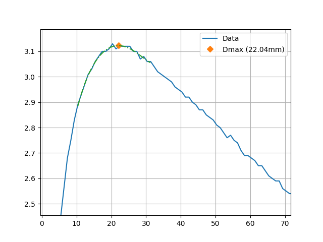
../_images/dmax.png — Zoomed in plot of a profile showing the polynomial fit used to find Dmax.¶

PDD¶

PDD This plugin calculates the percentage depth dose (PDD) of the profile at a given depth. A polynomial fit is performed around the desired depth and then the value of the polynomial at the desired depth is returned.

profile = FWXMProfile(...)
profile.compute(metrics=[PDD(depth_mm=100)])

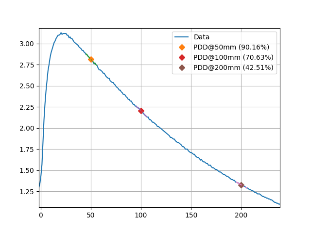
Ratio to Dmax¶

Since the PDD is a ratio of the maximum dose, the dmax is also calculated using, by default, a polynomial fit. I.e. if you ask for a PDD at 10 cm, two polynomial fits are done: one around 10 cm and one around the maximum and the ratio * 100 is the returned PDD. To override this behavior, set normalize_to='max'. Using max will simply normalize the depth value (still using a poly fit) to the maximum value of the profile.

Important

It is expected that the x-values of the profile are given in mm! I.e. FWXMProfile(..., x_values=...).

Accessing metrics¶

There are two ways to access the metrics calculated by a profile (what is returned by the metric’s calculate method). The first is what is returned by the compute method:

profile = FWXMProfile(...)
penum = profile.compute(metrics=PenumbraRightMetric())
print(penum)  # prints the penumbra value

We can also access the metric’s calculation by accessing the metric_values attribute of the profile:

profile = FWXMProfile(...)
profile.compute(metrics=[PenumbraRightMetric()])
print(profile.metric_values["Right Penumbra"])  # prints the penumbra value

Note

The key within a profile’s metric_values dictionary attribute is the value of the plugin’s name attribute.
Either 1 or multiple (as a list) metrics can be passed to the compute method.
There are metrics included in pylinac. See the built-in section.

Writing plugins¶

To write a plugin, create a class with the following conditions:

It inherits from ProfileMetric.
It implements a calculate() method that returns something.
It should also have a name attribute.

Note

This can be handled either by a class attribute or dynamically using a property.
(Optional) It implements a plot method can be declared that will plot the metric on the profile plot, although this is not required.

Note

Within the plugin, self.profile is available and will be the profile itself. This is so we can access the profile’s attributes and methods.
The calculate method can return anything, but a float is normal.
The plot method must take a matplotlib.plt.Axes object as an argument and return nothing. But a plot method is optional.

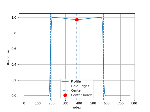
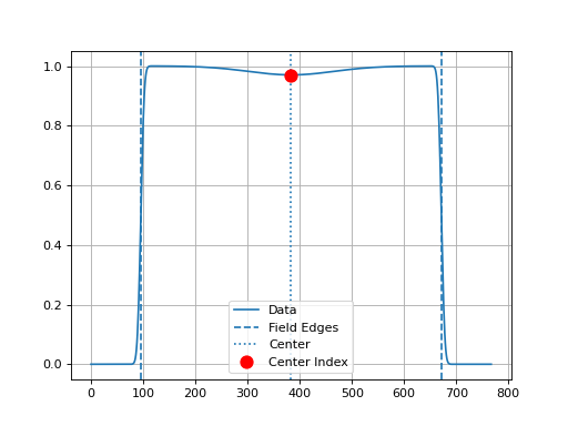
Center index example¶

For an example, let us write a plugin that calculates the value of the center index and also plots it.

import matplotlib.pyplot as plt

from pylinac.core.profile import ProfileMetric


class CenterMetric(ProfileMetric):
    name = "Center Index"  # human-readable string

    def calculate(self) -> float:
        """Return the index of the center of the profile."""
        return self.profile.center_idx

    def plot(self, axis: plt.Axes) -> None:
        """Plot the center index."""
        axis.plot(
            self.profile.center_idx,
            self.profile.y_at_x(self.profile.center_idx),
            "o",
            color="red",
            markersize=10,
            label=self.name,
        )

We can now pass this metric to the profile class’ compute method. We will use the image generator to create an image we will extract a profile from.

import matplotlib.pyplot as plt

from pylinac.core.profile import FWXMProfile, ProfileMetric
from pylinac.core.image_generator import AS1000Image, FilteredFieldLayer, GaussianFilterLayer
from pylinac.core.array_utils import normalize


# same as above; included so we can plot
class CenterMetric(ProfileMetric):
    name = 'Center Index'  # human-readable string

    def calculate(self) -> float:
        """Return the index of the center of the profile."""
        return self.profile.center_idx

    def plot(self, axis: plt.Axes) -> None:
        """Plot the center index."""
        axis.plot(self.profile.center_idx, self.profile.y_at_x(self.profile.center_idx), 'o', color='red',
                  markersize=10, label=self.name)

# this is our set up to get a nice profile
as1000 = AS1000Image()
as1000.add_layer(
    FilteredFieldLayer(field_size_mm=(100, 100))
)
as1000.add_layer(
    GaussianFilterLayer(sigma_mm=2)
)  # add an image-wide gaussian to simulate penumbra/scatter

# pull out the profile array
array = normalize(as1000.image[:, as1000.shape[1] // 2])

# create the profile
profile = FWXMProfile(array)

# compute the metric with our plugin
profile.compute(metrics=CenterMetric())

# plot the profile
profile.plot()

(Source code, png, hires.png, pdf)

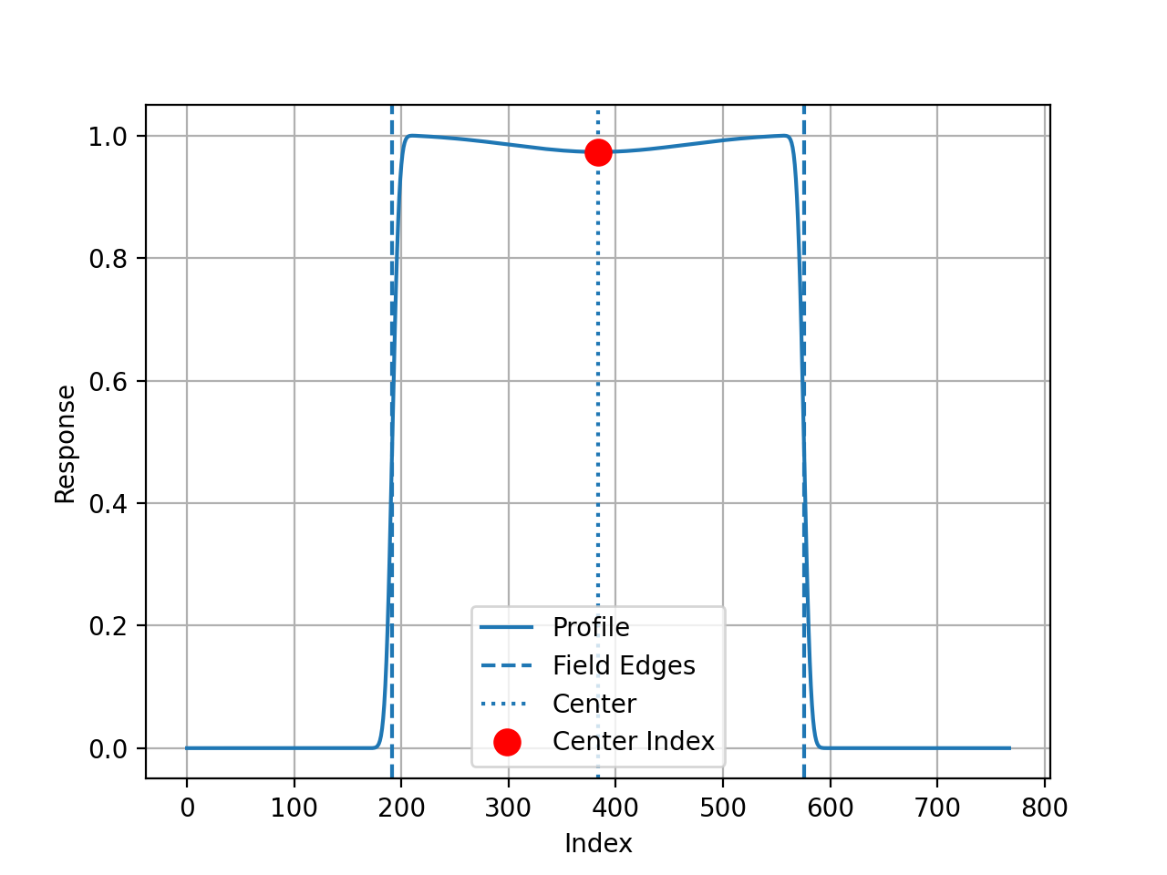
Resampling¶

Resampling a profile is the process of interpolating the profile data to a new resolution and can be done easily using as_resampled:

from pylinac.core.profile import FWXMProfilePhysical

profile = FWXMProfilePhysical(my_array, dpmm=3)
profile_resampled = profile.as_resampled(interpolation_resolution_mm=0.1)

This will create a new profile that is resampled to 0.1 mm resolution. The new profile’s dpmm attribute is also updated. The original profile is not modified.

Warning

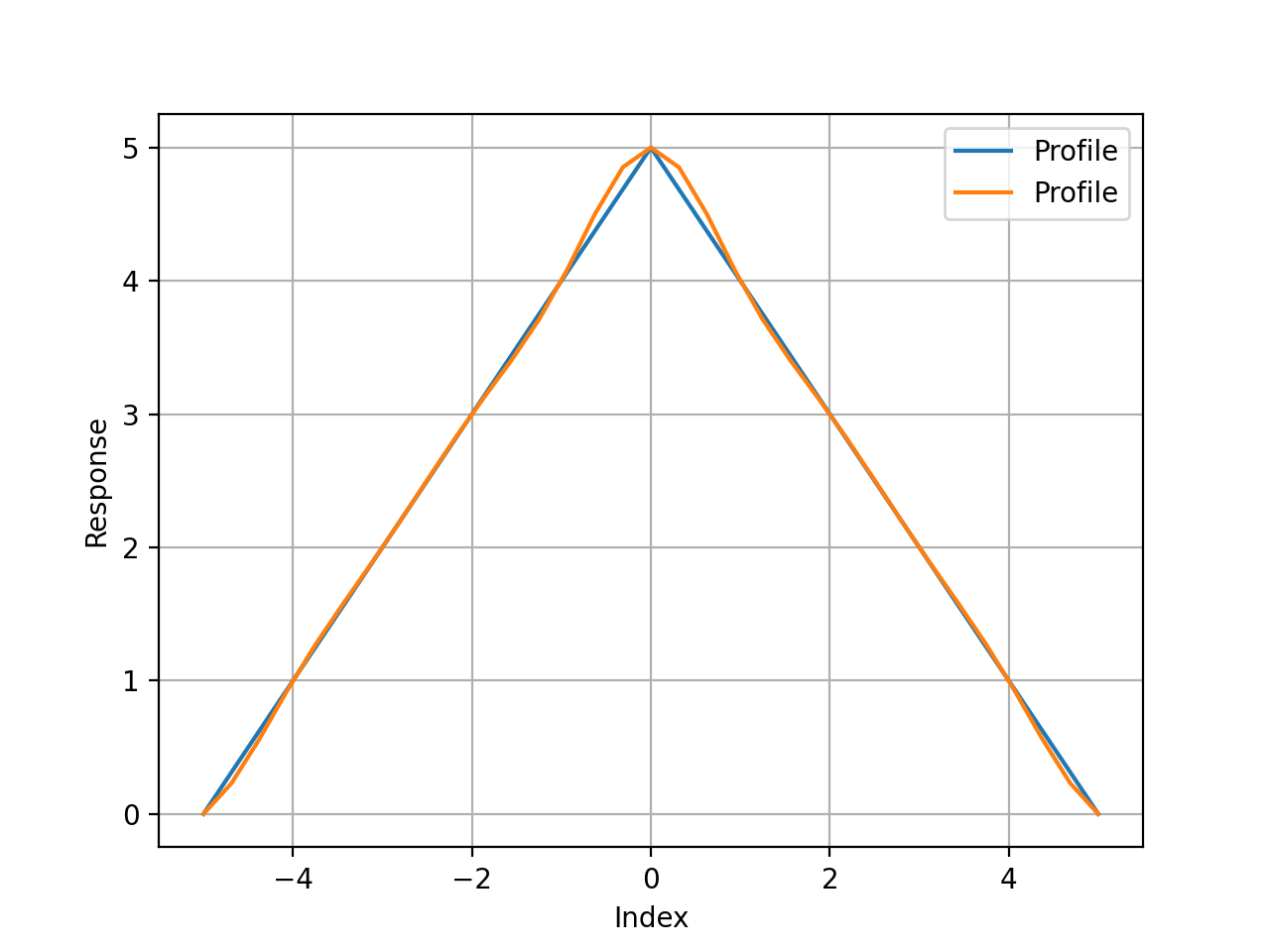
Resampling will respect the input datatype. If the array is an integer type and has a small range, the resampled array may be truncated. For example, if the array is an unsigned 16-bit integer (native EPID) and the range of values varies from 100 to 200, the resampled array will appear to be step-wise.

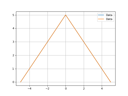
import numpy as np
from matplotlib import pyplot as plt

from pylinac.core.profile import FWXMProfile

y = np.array([0, 1, 2, 3, 4, 5, 4, 3, 2, 1, 0], dtype=int)
x = np.array([-5, -4, -3, -2, -1, 0, 1, 2, 3, 4, 5], dtype=int)

prof = FWXMProfile(values=y, x_values=x)
prof_interp = prof.as_resampled(interpolation_factor=2)
ax = prof.plot(show=False, show_field_edges=False, show_center=False)
prof_interp.plot(show=True, axis=ax, show_field_edges=False, show_center=False)

(Source code, png, hires.png, pdf)

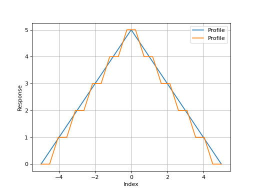
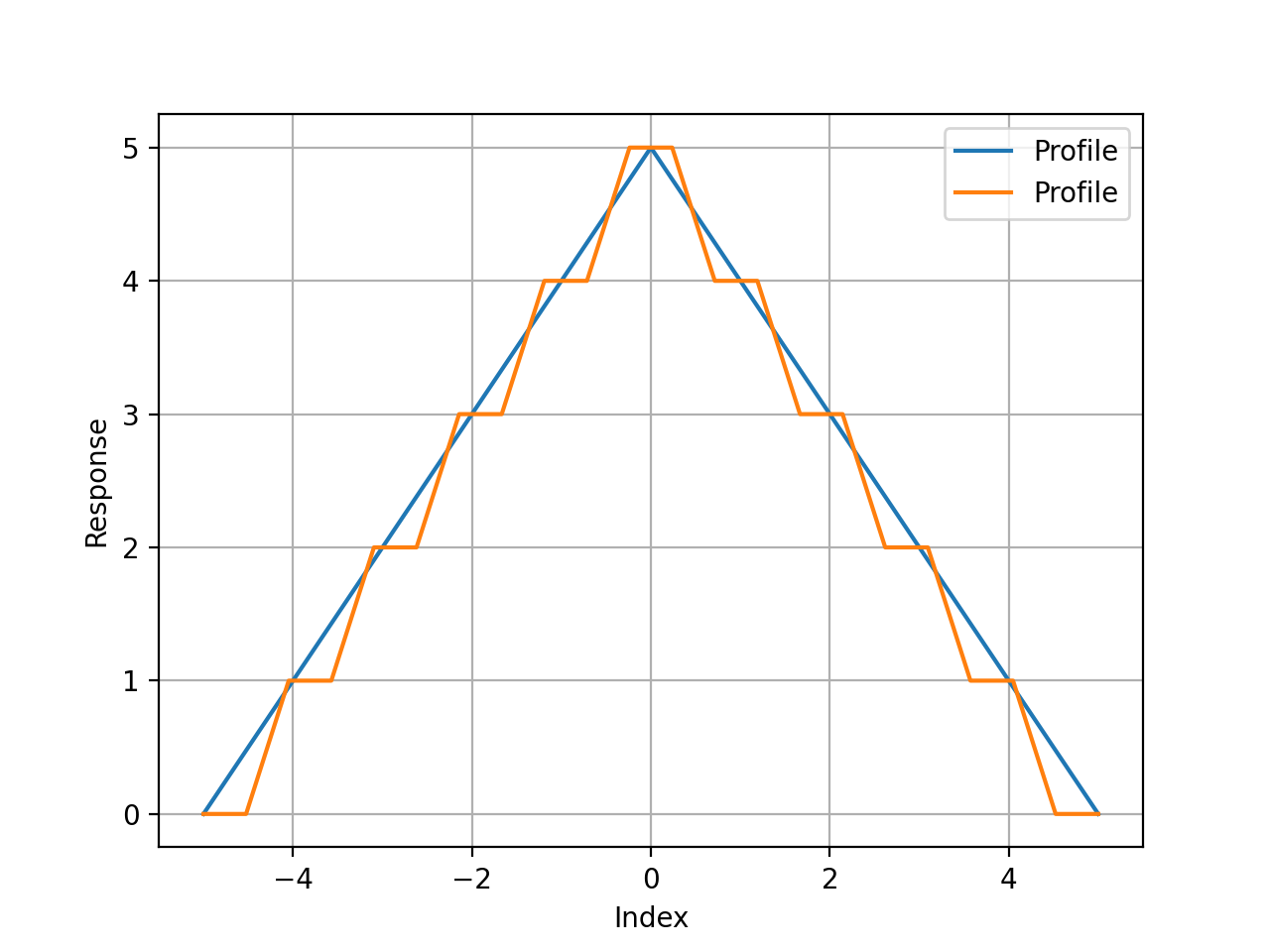
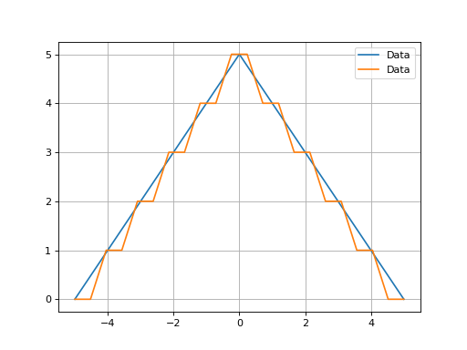
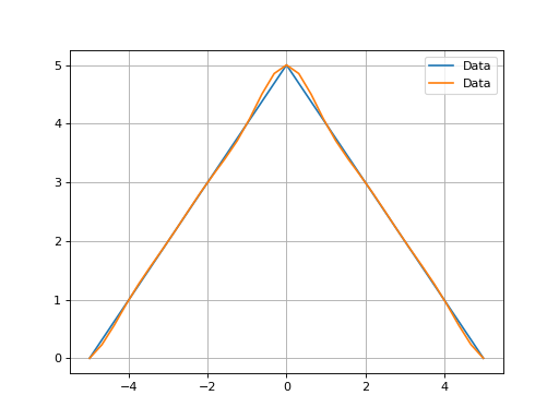
Compare this to a float array:

import numpy as np
from matplotlib import pyplot as plt

from pylinac.core.profile import FWXMProfile

y = np.array([0, 1, 2, 3, 4, 5, 4, 3, 2, 1, 0], dtype=float)
x = np.array([-5, -4, -3, -2, -1, 0, 1, 2, 3, 4, 5], dtype=float)

prof = FWXMProfile(values=y, x_values=x)
prof_interp = prof.as_resampled(interpolation_factor=2)
ax = prof.plot(show=False, show_field_edges=False, show_center=False)
prof_interp.plot(show=True, axis=ax, show_field_edges=False, show_center=False)

(Source code, png, hires.png, pdf)

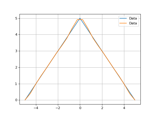
This float array is interpolated better, although there is still some apparent spline interpolation fit error.

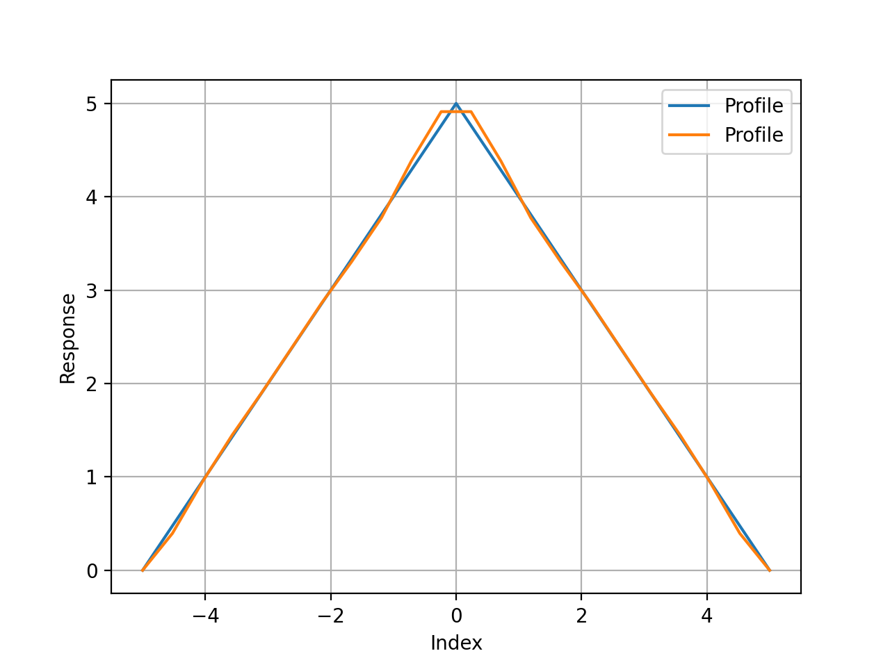
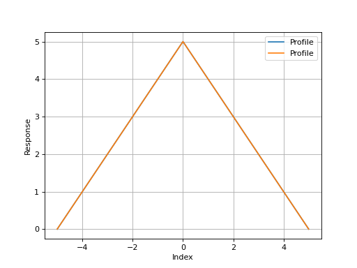
This second issue can be resolved by using an odd-sized interpolation factor:

import numpy as np
from matplotlib import pyplot as plt

from pylinac.core.profile import FWXMProfile

y = np.array([0, 1, 2, 3, 4, 5, 4, 3, 2, 1, 0], dtype=float)
x = np.array([-5, -4, -3, -2, -1, 0, 1, 2, 3, 4, 5], dtype=float)

prof = FWXMProfile(values=y, x_values=x)
prof_interp = prof.as_resampled(interpolation_factor=3)  # not 2
ax = prof.plot(show=False, show_field_edges=False, show_center=False)
prof_interp.plot(show=True, axis=ax, show_field_edges=False, show_center=False)

(Source code, png, hires.png, pdf)

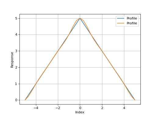
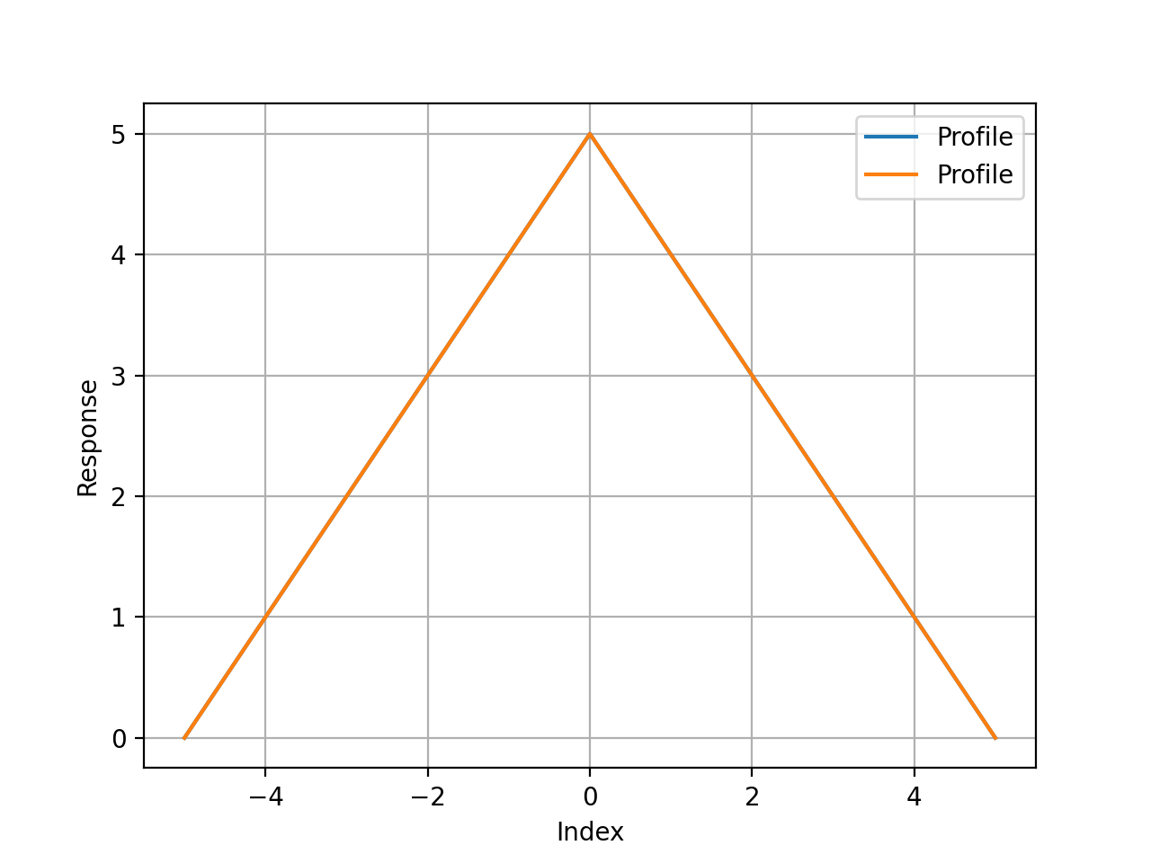
Better, but still not perfect. Most profiles do not look like this however. This is an extreme example. However, even here we can improve things by using linear interpolation. This is done by setting the order parameter to 1:

import numpy as np
from matplotlib import pyplot as plt

from pylinac.core.profile import FWXMProfile

y = np.array([0, 1, 2, 3, 4, 5, 4, 3, 2, 1, 0], dtype=float)
x = np.array([-5, -4, -3, -2, -1, 0, 1, 2, 3, 4, 5], dtype=float)

prof = FWXMProfile(values=y, x_values=x)
prof_interp = prof.as_resampled(interpolation_factor=3, order=1)  # order=1 => linear
ax = prof.plot(show=False, show_field_edges=False, show_center=False)
prof_interp.plot(show=True, axis=ax, show_field_edges=False, show_center=False)

(Source code, png, hires.png, pdf)

Note

Resampling can be used for both upsampling and downsampling.

Important

The parameters for as_resampled are slightly different between the physical and non-physical classes. For physical classes, the new resolution is in mm/pixels. For non-physical classes, the new resolution is a simple factor like 5x or 10x the original resolution.

Important

Resampling is not the same as smoothing. Smoothing is the process of removing noise from the profile. Resampling is the process of changing the resolution of the profile. To apply a filter, use the filter() method:

from pylinac.core.profile import FWXMProfile

profile = FWXMProfile(...)
profile.filter(size=5, kind="gaussian")

Warning

When resampling a physical profile, it is important to know that interpolation must account for the physical size of the pixels and how that affects the edge of the array. Simply resampling the array without accounting for the physical size of the pixels will result in a profile that is not accurate at the edges. The simplest way to visualize this is shown in the grid_mode parameter of scipy’s zoom function.

Multiple resampling¶

Profiles can be resampled multiple times, but it is important to set grid_mode=False on secondary resamplings. This is because the physical size of the pixels is already accounted for in the first resampling. If grid_mode=True is used on secondary resamplings, the profile edges will not accurately represent the physical size and position of the pixels:

from pylinac.core.profile import FWXMProfilePhysical

profile = FWXMProfilePhysical(my_array, dpmm=3)
profile_resampled = profile.as_resampled(interpolation_resolution_mm=0.1)
# use grid_mode=False on secondary resamplings
profile_resampled2 = profile_resampled.as_resampled(
    interpolation_resolution_mm=0.05, grid_mode=False
)

# if we resample to 0.05mm directly from the original it will be the same as the above
profile_resampled3 = profile.as_resampled(interpolation_resolution_mm=0.05)
assert len(profile_resampled2) == len(profile_resampled3)
# assert the left edge is at the same physical location
assert profile_resampled2.x_values[0] == profile_resampled3.x_values[0]

API¶

class pylinac.core.profile.SingleProfile(values: ndarray, dpmm: float = None, interpolation: Interpolation | str | None = Interpolation.LINEAR, ground: bool = True, interpolation_resolution_mm: float = 0.1, interpolation_factor: float = 10, normalization_method: Normalization | str = Normalization.BEAM_CENTER, edge_detection_method: Edge | str = Edge.FWHM, edge_smoothing_ratio: float = 0.003, hill_window_ratio: float = 0.1, x_values: ndarray | None = None)[source]¶

Bases: ProfileMixin

A profile that has one large signal, e.g. a radiation beam profile. Signal analysis methods are given, mostly based on FWXM and on Hill function calculations. Profiles with multiple peaks are better suited by the MultiProfile class.

Parameters¶

values

The profile numpy array. Must be 1D.

dpmm

The dots (pixels) per mm. Pass to get info like beam width in distance units in addition to pixels

interpolation

Interpolation technique.

ground

Whether to ground the profile (set min value to 0). Helpful most of the time.

interpolation_resolution_mm

The resolution that the interpolation will scale to. Only used if dpmm is passed and interpolation is set. E.g. if the dpmm is 0.5 and the resolution is set to 0.1mm the data will be interpolated to have a new dpmm of 10 (1/0.1).

interpolation_factor

The factor to multiply the data by. Only used if interpolation is used and dpmm is NOT passed. E.g. 10 will perfectly decimate the existing data according to the interpolation method passed.

normalization_method

How to pick the point to normalize the data to.

edge_detection_method

The method by which to detect the field edge. FWHM is reasonable most of the time except for FFF beams. Inflection-derivative will use the max gradient to determine the field edge. Note that this may not be the 50% height. In fact, for FFF beams it shouldn’t be. Inflection methods are better for FFF and other unusual beam shapes.

edge_smoothing_ratio

Only applies to INFLECTION_DERIVATIVE and INFLECTION_HILL.

The ratio of the length of the values to use as the sigma for a Gaussian filter applied before searching for the inflection. E.g. 0.005 with a profile of 1000 points will result in a sigma of 5. This helps make the inflection point detection more robust to noise. Increase for noisy data.

hill_window_ratio

The ratio of the field size to use as the window to fit the Hill function. E.g. 0.2 will using a window centered about each edge with a width of 20% the size of the field width. Only applies when the edge detection is INFLECTION_HILL.

x_values

The x-values of the profile, if any. If None, will generate a simple range(len(values)).

resample(interpolation_factor: int = 10, interpolation_resolution_mm: float = 0.1) → SingleProfile[source]¶: Resample the profile at a new resolution. Returns a new profile

geometric_center() → dict[source]¶: The geometric center (i.e. the device center)

beam_center() → dict[source]¶: The center of the detected beam. This can account for asymmetries in the beam position (e.g. offset jaws)

fwxm_data(x: int = 50) → dict[source]¶

Return the width at X-Max, where X is the percentage height.

Parameters¶

x: The percent height of the profile. E.g. x = 50 is 50% height, i.e. FWHM.

field_data(in_field_ratio: float = 0.8, slope_exclusion_ratio=0.2) → dict[source]¶

Return the width at X-Max, where X is the percentage height.

Parameters¶

in_field_ratio: In Field Ratio: 1.0 is the entire detected field; 0.8 would be the central 80%, etc.
slope_exclusion_ratio: Ratio of the field width to use as the cutoff between “top” calculation and “slope” calculation. Useful for FFF beams. This area is centrally located in the field. E.g. 0.2 will use the central 20% of the field to calculate the “top” value. To calculate the slope of each side, the field width between the edges of the in_field_ratio and the slope exclusion region are used.

Warning

The “top” value is always calculated. For FFF beams this should be reasonable, but for flat beams this value may end up being non-sensible.

inflection_data() → dict[source]¶: Calculate the profile inflection values using either the 2nd derivative or a fitted Hill function.

Note

This only applies if the edge detection method is INFLECTION_….

Parameters¶

penumbra(lower: int = 20, upper: int = 80)[source]¶

Calculate the penumbra of the field. Dependent on the edge detection method.

Parameters¶

lower: The lower % of the beam to use. If the edge method is FWHM, this is the typical % penumbra you’re thinking. If the inflection method is used it will be the value/50 of the inflection point value. E.g. if the inflection point is perfectly at 50% with a lower of 20, then the penumbra value here will be 20% of the maximum. If the inflection point is at 30% of the max value (say for a FFF beam) then the lower penumbra will be lower/50 of the inflection point or 0.3*lower/50.
upper: Upper % of the beam to use. See lower for details.

field_calculation(in_field_ratio: float = 0.8, calculation: str = 'mean', slope_exclusion_ratio: float = 0.2) → float | tuple[float, float][source]¶

Perform an operation on the field values of the profile. This function is useful for determining field symmetry and flatness.

Parameters¶

in_field_ratio: Ratio of the field width to use in the calculation.
calculation{‘mean’, ‘median’, ‘max’, ‘min’, ‘area’}: Calculation to perform on the field values.

gamma(evaluation_profile: SingleProfile, distance_to_agreement: float = 1, dose_to_agreement: float = 1, gamma_cap_value: float = 2, dose_threshold: float = 5, global_dose: bool = True, fill_value: float = nan) → ndarray[source]¶

Calculate a 1D gamma. The passed profile is the evaluation profile. The instance calling this method is the reference profile. This profile must have the dpmm value given at instantiation so that physical spacing can be evaluated. The evaluation profile is resampled to be the same resolution as the reference profile.

Note

The difference between this method and the gamma_1d function is that 1) this is computed on Profile instances and 2) this validates the physical spacing of the profiles.

Parameters¶

evaluation_profile: The evaluation profile. This profile must have the dpmm value given at instantiation so that physical spacing can be evaluated.
distance_to_agreement: Distance in mm to search
dose_to_agreement: Dose in % of either global or local reference dose
gamma_cap_value: The value to cap the gamma at. E.g. a gamma of 5.3 will get capped to 2. Useful for displaying data with a consistent range.
global_dose: Whether to evaluate the dose to agreement threshold based on the global max or the dose point under evaluation.
dose_threshold: The dose threshold as a number between 0 and 100 of the % of max dose under which a gamma is not calculated. This is not affected by the global/local dose normalization and the threshold value is evaluated against the global max dose, period.
fill_value: The value to give pixels that were not calculated because they were under the dose threshold. Default is NaN, but another option would be 0. If NaN, allows the user to calculate mean/median gamma over just the evaluated portion and not be skewed by 0’s that should not be considered.

plot(show: bool = True) → None[source]¶: Plot the profile.

bit_invert() → None¶: Invert the profile bit-wise.

convert_to_dtype(dtype: type[dtype]) → None¶: Convert the profile datatype to another datatype while retaining the values relative to the datatype min/max

filter(size: float = 0.05, kind: str = 'median') → None¶

Filter the profile.

Parameters¶

sizefloat, int: Size of the median filter to apply. If a float, the size is the ratio of the length. Must be in the range 0-1. E.g. if size=0.1 for a 1000-element array, the filter will be 100 elements. If an int, the filter is the size passed.
kind{‘median’, ‘gaussian’}: The kind of filter to apply. If gaussian, size is the sigma value.

ground() → float¶

Ground the profile such that the lowest value is 0.

Returns¶

float: The minimum value that was used as the grounding value.

invert() → None¶: Invert the profile.

normalize(norm_val: str | float | None = None) → None¶

Normalize the profile to the given value.

Parameters¶

norm_valnumber or ‘max’ or None: If a number, normalize the array to that number. If None, normalizes to the maximum value.

stretch(min: float = 0, max: float = 1) → None¶

‘Stretch’ the profile to the min and max parameter values.

Parameters¶

minnumber: The new minimum of the values
maxnumber: The new maximum value.

class pylinac.core.profile.FWXMProfile(values: np.array, x_values: np.array | None = None, ground: bool = False, normalization: str | Normalization = Normalization.NONE, fwxm_height: float = 50)[source]¶

Bases: ProfileBase

A profile that has one large signal, e.g. a radiation beam profile and data derived from it is based on the Full-Width X-Maximum to find the edge indices

A 1D profile that has one large signal, e.g. a radiation beam profile. Signal analysis methods are given, mostly based on FWXM and on Hill function calculations. Profiles with multiple peaks are better suited by the MultiProfile class.

field_edge_idx(side: Literal['right', 'left']) → float[source]¶: The edge index of the given side using the FWXM methodology

as_resampled(interpolation_factor: float = 10, order: int = 3) → FWXMProfile[source]¶

Resample the profile at a new resolution. Returns a new profile.

Parameters¶

interpolation_factorfloat: The factor to zoom the profile by. E.g. 10 means the profile will be 10x larger.
orderint: The order of the spline interpolation. 1 is linear, 3 is cubic, etc.

bit_invert() → None¶: Invert the profile bit-wise.

property center_idx: float¶: The center index of the profile. Halfway between the field edges.

compute(metrics: Iterable[ProfileMetric] | ProfileMetric) → Any | dict[str, Any]¶

Compute metric(s) on the profile.

Unlike other modules, calling compute is not strictly necessary. Only call it if there are metrics to calculate.

Parameters¶

metrics: iterable of ProfileMetric | ProfileMetric: List of metrics to calculate. If only one metric is desired, it can be passed directly.

Returns¶

dict | list: A dictionary of metric names and values if multiple metrics were given. If only one metric was given, the value of that metric is returned.

convert_to_dtype(dtype: type[dtype]) → None¶: Convert the profile datatype to another datatype while retaining the values relative to the datatype min/max

field_indices(in_field_ratio: float)¶: Return the indices of the left and right edge of the field, given the in-field ratio. Importantly, this will use the same rounding behavior as field_values.

field_values(in_field_ratio: float = 0.8) → ndarray¶: The array of values of the profile within the ‘field’ area. This is typically 80% of the detected field width.

property field_width_px: float¶: The field width of the profile in pixels

field_x_values(in_field_ratio: float) → ndarray¶: Return the x-values of the field, given the in-field ratio. This is helpful when plotting the field to include the proper x-values as well.

filter(size: float = 0.05, kind: str = 'median') → None¶

Filter the profile.

Parameters¶

sizefloat, int: Size of the median filter to apply. If a float, the size is the ratio of the length. Must be in the range 0-1. E.g. if size=0.1 for a 1000-element array, the filter will be 100 elements. If an int, the filter is the size passed.
kind{‘median’, ‘gaussian’}: The kind of filter to apply. If gaussian, size is the sigma value.

ground() → float¶

Ground the profile such that the lowest value is 0.

Returns¶

float: The minimum value that was used as the grounding value.

invert() → None¶: Invert the profile.

normalize(norm_val: str | float | None = None) → None¶

Normalize the profile to the given value.

Parameters¶

norm_valnumber or ‘max’ or None: If a number, normalize the array to that number. If None, normalizes to the maximum value.

plot(show: bool = True, axis: Axes | None = None, show_field_edges: bool = True, show_grid: bool = True, show_center: bool = True) → Axes¶: Plot the profile along with relevant overlays to point out features.

resample_to(target_profile: ProfileBase | PhysicalProfileMixin) → ProfileBase¶

Resample a target profile to have the same sampling (x-values) rate as the source profile. This will return a new target profile with the same x-values as the source profile and with the values interpolated to match the source profile.

For example, this can be used to resample an EPID profile to have the same sampling rate as an ion chamber profile or vice versa.

Requirements¶

The range of x-values for the target profile must be within the x-value range of the source profile. I.e. no extrapolation of the source profile. For example, if we have a profile of an IC Profile, that goes from -15cm to +15cm, we cannot resample onto an EPID profile that goes from -20cm to +20cm. To do so, go the other way: resample the EPID profile onto the IC profile.

stretch(min: float = 0, max: float = 1) → None¶

‘Stretch’ the profile to the min and max parameter values.

Parameters¶

minnumber: The new minimum of the values
maxnumber: The new maximum value.

x_at_x(x: float) → ndarray¶: Deprecated alias for x_at_x_idx

x_at_x_idx(x: float | ndarray) → ndarray | float¶: Return the physical x-value at the given index. When no x-values are provided, these are the same. However, physical dimensions can be different than the index.

x_at_y(y: float | ndarray, side: str) → ndarray | float¶: Interpolated y-values. Can use floats as indices.

x_idx_at_x(x: float) → int¶: Return the index of the x-value closest to the given x-value.

y_at_x(x: float | ndarray) → ndarray | float¶: Interpolated y-values. The x-value is the physical position, not the index. However, if no x-values were provided, these will be the same.

class pylinac.core.profile.FWXMProfilePhysical(values: np.array, dpmm: float, x_values: np.array | None = None, ground: bool = False, normalization: str | Normalization = Normalization.NONE, fwxm_height: float = 50)[source]¶

Bases: PhysicalProfileMixin, FWXMProfile

as_resampled(interpolation_resolution_mm: float = 0.1, order: int = 3, grid: bool = True) → FWXMProfilePhysical[source]¶

Resample the physical profile at a new resolution. Returns a new profile.

Parameters¶

interpolation_resolution_mmfloat: The resolution to resample to in mm. E.g. 0.1 means the profile will be 0.1 mm resolution.
orderint: The order of the spline interpolation. 1 is linear, 3 is cubic, etc.
gridbool: Whether to use grid mode when zooming. See parameter grid_mode in zoom() for more information. This should be true unless you are resampling an already-resampled physical array.

Warnings¶

This method will respect the input datatype of the numpy array. If the input array is a float, the output array will be a float. This can cause issues for int arrays with a small range. E.g. if the range is only 10, interpolation will look more step-like than smooth. If this is the case, convert the array to a float before passing it to this method. The array is not automatically converted to float in this case to respect the original dtype. However, a warning will be produced.

as_simple_profile() → ProfileBase¶

Convert a physical profile into a simple profile where the x-values have been converted to the physical x-values.

An example is converting an EPID profile into a simple profile where the x-values are in mm, not pixels.

This can be useful when trying to compare physical profiles to simple profiles. E.g. an EPID vs an ion chamber profile acquisition. In the EPID’s case, the x-values are indices w/ a dpmm component. The IC profile is usually already directly in absolute x-values.

bit_invert() → None¶: Invert the profile bit-wise.

property center_idx: float¶: The center index of the profile. Halfway between the field edges.

compute(metrics: Iterable[ProfileMetric] | ProfileMetric) → Any | dict[str, Any]¶

Compute metric(s) on the profile.

Unlike other modules, calling compute is not strictly necessary. Only call it if there are metrics to calculate.

Parameters¶

metrics: iterable of ProfileMetric | ProfileMetric: List of metrics to calculate. If only one metric is desired, it can be passed directly.

Returns¶

dict | list: A dictionary of metric names and values if multiple metrics were given. If only one metric was given, the value of that metric is returned.

convert_to_dtype(dtype: type[dtype]) → None¶: Convert the profile datatype to another datatype while retaining the values relative to the datatype min/max

field_edge_idx(side: Literal['right', 'left']) → float¶: The edge index of the given side using the FWXM methodology

field_indices(in_field_ratio: float)¶: Return the indices of the left and right edge of the field, given the in-field ratio. Importantly, this will use the same rounding behavior as field_values.

field_values(in_field_ratio: float = 0.8) → ndarray¶: The array of values of the profile within the ‘field’ area. This is typically 80% of the detected field width.

property field_width_mm: float¶: The field width of the profile in mm

property field_width_px: float¶: The field width of the profile in pixels

field_x_values(in_field_ratio: float) → ndarray¶: Return the x-values of the field, given the in-field ratio. This is helpful when plotting the field to include the proper x-values as well.

filter(size: float = 0.05, kind: str = 'median') → None¶

Filter the profile.

Parameters¶

sizefloat, int: Size of the median filter to apply. If a float, the size is the ratio of the length. Must be in the range 0-1. E.g. if size=0.1 for a 1000-element array, the filter will be 100 elements. If an int, the filter is the size passed.
kind{‘median’, ‘gaussian’}: The kind of filter to apply. If gaussian, size is the sigma value.

ground() → float¶

Ground the profile such that the lowest value is 0.

Returns¶

float: The minimum value that was used as the grounding value.

invert() → None¶: Invert the profile.

normalize(norm_val: str | float | None = None) → None¶

Normalize the profile to the given value.

Parameters¶

norm_valnumber or ‘max’ or None: If a number, normalize the array to that number. If None, normalizes to the maximum value.

property physical_x_values: array¶: The x-values of the profile in absolute position, taking into account the dpmm.

plot(show: bool = True, axis: Axes | None = None, show_field_edges: bool = True, show_grid: bool = True, show_center: bool = True) → Axes¶: Plot the profile along with relevant overlays to point out features.

resample_to(target_profile: ProfileBase | PhysicalProfileMixin) → ProfileBase¶

For example, this can be used to resample an EPID profile to have the same sampling rate as an ion chamber profile or vice versa.

Requirements¶

The range of x-values for the target profile must be within the x-value range of the source profile. I.e. no extrapolation of the source profile. For example, if we have a profile of an IC Profile, that goes from -15cm to +15cm, we cannot resample onto an EPID profile that goes from -20cm to +20cm. To do so, go the other way: resample the EPID profile onto the IC profile.

stretch(min: float = 0, max: float = 1) → None¶

‘Stretch’ the profile to the min and max parameter values.

Parameters¶

minnumber: The new minimum of the values
maxnumber: The new maximum value.

x_at_x(x: float) → ndarray¶: Deprecated alias for x_at_x_idx

x_at_x_idx(x: float | ndarray) → ndarray | float¶: Return the physical x-value at the given index. When no x-values are provided, these are the same. However, physical dimensions can be different than the index.

x_at_y(y: float | ndarray, side: str) → ndarray | float¶: Interpolated y-values. Can use floats as indices.

x_idx_at_x(x: float) → int¶: Return the index of the x-value closest to the given x-value.

y_at_x(x: float | ndarray) → ndarray | float¶: Interpolated y-values. The x-value is the physical position, not the index. However, if no x-values were provided, these will be the same.

class pylinac.core.profile.InflectionDerivativeProfile(values: np.array, x_values: np.array | None = None, ground: bool = False, normalization: str | Normalization = Normalization.NONE, edge_smoothing_ratio: float = 0.003)[source]¶

Bases: ProfileBase

A profile that has one large signal, e.g. a radiation beam profile and data derived from it is based on the Full-Width X-Maximum

field_edge_idx(side: str) → float[source]¶: The edge index of the given side using the second derivative methodology

as_resampled(interpolation_factor: float = 10, order: int = 3) → InflectionDerivativeProfile[source]¶

Resample the profile at a new resolution. Returns a new profile.

Parameters¶

interpolation_factorfloat: The factor to zoom the profile by. E.g. 10 means the profile will be 10x larger.
orderint: The order of the spline interpolation. 1 is linear, 3 is cubic, etc.

Warnings¶

bit_invert() → None¶: Invert the profile bit-wise.

property center_idx: float¶: The center index of the profile. Halfway between the field edges.

compute(metrics: Iterable[ProfileMetric] | ProfileMetric) → Any | dict[str, Any]¶

Compute metric(s) on the profile.

Unlike other modules, calling compute is not strictly necessary. Only call it if there are metrics to calculate.

Parameters¶

metrics: iterable of ProfileMetric | ProfileMetric: List of metrics to calculate. If only one metric is desired, it can be passed directly.

Returns¶

dict | list: A dictionary of metric names and values if multiple metrics were given. If only one metric was given, the value of that metric is returned.

convert_to_dtype(dtype: type[dtype]) → None¶: Convert the profile datatype to another datatype while retaining the values relative to the datatype min/max

field_indices(in_field_ratio: float)¶: Return the indices of the left and right edge of the field, given the in-field ratio. Importantly, this will use the same rounding behavior as field_values.

field_values(in_field_ratio: float = 0.8) → ndarray¶: The array of values of the profile within the ‘field’ area. This is typically 80% of the detected field width.

property field_width_px: float¶: The field width of the profile in pixels

field_x_values(in_field_ratio: float) → ndarray¶: Return the x-values of the field, given the in-field ratio. This is helpful when plotting the field to include the proper x-values as well.

filter(size: float = 0.05, kind: str = 'median') → None¶

Filter the profile.

Parameters¶

sizefloat, int: Size of the median filter to apply. If a float, the size is the ratio of the length. Must be in the range 0-1. E.g. if size=0.1 for a 1000-element array, the filter will be 100 elements. If an int, the filter is the size passed.
kind{‘median’, ‘gaussian’}: The kind of filter to apply. If gaussian, size is the sigma value.

ground() → float¶

Ground the profile such that the lowest value is 0.

Returns¶

float: The minimum value that was used as the grounding value.

invert() → None¶: Invert the profile.

normalize(norm_val: str | float | None = None) → None¶

Normalize the profile to the given value.

Parameters¶

norm_valnumber or ‘max’ or None: If a number, normalize the array to that number. If None, normalizes to the maximum value.

plot(show: bool = True, axis: Axes | None = None, show_field_edges: bool = True, show_grid: bool = True, show_center: bool = True) → Axes¶: Plot the profile along with relevant overlays to point out features.

resample_to(target_profile: ProfileBase | PhysicalProfileMixin) → ProfileBase¶

For example, this can be used to resample an EPID profile to have the same sampling rate as an ion chamber profile or vice versa.

Requirements¶

The range of x-values for the target profile must be within the x-value range of the source profile. I.e. no extrapolation of the source profile. For example, if we have a profile of an IC Profile, that goes from -15cm to +15cm, we cannot resample onto an EPID profile that goes from -20cm to +20cm. To do so, go the other way: resample the EPID profile onto the IC profile.

stretch(min: float = 0, max: float = 1) → None¶

‘Stretch’ the profile to the min and max parameter values.

Parameters¶

minnumber: The new minimum of the values
maxnumber: The new maximum value.

x_at_x(x: float) → ndarray¶: Deprecated alias for x_at_x_idx

x_at_x_idx(x: float | ndarray) → ndarray | float¶: Return the physical x-value at the given index. When no x-values are provided, these are the same. However, physical dimensions can be different than the index.

x_at_y(y: float | ndarray, side: str) → ndarray | float¶: Interpolated y-values. Can use floats as indices.

x_idx_at_x(x: float) → int¶: Return the index of the x-value closest to the given x-value.

y_at_x(x: float | ndarray) → ndarray | float¶: Interpolated y-values. The x-value is the physical position, not the index. However, if no x-values were provided, these will be the same.

class pylinac.core.profile.InflectionDerivativeProfilePhysical(values: np.array, dpmm: float, x_values: np.array | None = None, ground: bool = False, normalization: str | Normalization = Normalization.NONE, edge_smoothing_ratio: float = 0.003)[source]¶

Bases: PhysicalProfileMixin, InflectionDerivativeProfile

as_resampled(interpolation_resolution_mm: float = 0.1, order: int = 3, grid: bool = True) → InflectionDerivativeProfilePhysical[source]¶

Resample the physical profile at a new resolution. Returns a new profile.

Parameters¶

interpolation_resolution_mmfloat: The resolution to resample to in mm. E.g. 0.1 means the profile will be 0.1 mm resolution.
orderint: The order of the spline interpolation. 1 is linear, 3 is cubic, etc.
gridbool: Whether to use grid mode when zooming. See parameter grid_mode in zoom() for more information. This should be true unless you are resampling an already-resampled physical array.

Warnings¶

as_simple_profile() → ProfileBase¶

Convert a physical profile into a simple profile where the x-values have been converted to the physical x-values.

An example is converting an EPID profile into a simple profile where the x-values are in mm, not pixels.

bit_invert() → None¶: Invert the profile bit-wise.

property center_idx: float¶: The center index of the profile. Halfway between the field edges.

compute(metrics: Iterable[ProfileMetric] | ProfileMetric) → Any | dict[str, Any]¶

Compute metric(s) on the profile.

Unlike other modules, calling compute is not strictly necessary. Only call it if there are metrics to calculate.

Parameters¶

metrics: iterable of ProfileMetric | ProfileMetric: List of metrics to calculate. If only one metric is desired, it can be passed directly.

Returns¶

dict | list: A dictionary of metric names and values if multiple metrics were given. If only one metric was given, the value of that metric is returned.

convert_to_dtype(dtype: type[dtype]) → None¶: Convert the profile datatype to another datatype while retaining the values relative to the datatype min/max

field_edge_idx(side: str) → float¶: The edge index of the given side using the second derivative methodology

field_indices(in_field_ratio: float)¶: Return the indices of the left and right edge of the field, given the in-field ratio. Importantly, this will use the same rounding behavior as field_values.

field_values(in_field_ratio: float = 0.8) → ndarray¶: The array of values of the profile within the ‘field’ area. This is typically 80% of the detected field width.

property field_width_mm: float¶: The field width of the profile in mm

property field_width_px: float¶: The field width of the profile in pixels

field_x_values(in_field_ratio: float) → ndarray¶: Return the x-values of the field, given the in-field ratio. This is helpful when plotting the field to include the proper x-values as well.

filter(size: float = 0.05, kind: str = 'median') → None¶

Filter the profile.

Parameters¶

sizefloat, int: Size of the median filter to apply. If a float, the size is the ratio of the length. Must be in the range 0-1. E.g. if size=0.1 for a 1000-element array, the filter will be 100 elements. If an int, the filter is the size passed.
kind{‘median’, ‘gaussian’}: The kind of filter to apply. If gaussian, size is the sigma value.

ground() → float¶

Ground the profile such that the lowest value is 0.

Returns¶

float: The minimum value that was used as the grounding value.

invert() → None¶: Invert the profile.

normalize(norm_val: str | float | None = None) → None¶

Normalize the profile to the given value.

Parameters¶

norm_valnumber or ‘max’ or None: If a number, normalize the array to that number. If None, normalizes to the maximum value.

property physical_x_values: array¶: The x-values of the profile in absolute position, taking into account the dpmm.

plot(show: bool = True, axis: Axes | None = None, show_field_edges: bool = True, show_grid: bool = True, show_center: bool = True) → Axes¶: Plot the profile along with relevant overlays to point out features.

resample_to(target_profile: ProfileBase | PhysicalProfileMixin) → ProfileBase¶

For example, this can be used to resample an EPID profile to have the same sampling rate as an ion chamber profile or vice versa.

Requirements¶

The range of x-values for the target profile must be within the x-value range of the source profile. I.e. no extrapolation of the source profile. For example, if we have a profile of an IC Profile, that goes from -15cm to +15cm, we cannot resample onto an EPID profile that goes from -20cm to +20cm. To do so, go the other way: resample the EPID profile onto the IC profile.

stretch(min: float = 0, max: float = 1) → None¶

‘Stretch’ the profile to the min and max parameter values.

Parameters¶

minnumber: The new minimum of the values
maxnumber: The new maximum value.

x_at_x(x: float) → ndarray¶: Deprecated alias for x_at_x_idx

x_at_x_idx(x: float | ndarray) → ndarray | float¶: Return the physical x-value at the given index. When no x-values are provided, these are the same. However, physical dimensions can be different than the index.

x_at_y(y: float | ndarray, side: str) → ndarray | float¶: Interpolated y-values. Can use floats as indices.

x_idx_at_x(x: float) → int¶: Return the index of the x-value closest to the given x-value.

y_at_x(x: float | ndarray) → ndarray | float¶: Interpolated y-values. The x-value is the physical position, not the index. However, if no x-values were provided, these will be the same.

class pylinac.core.profile.HillProfile(values: np.array, x_values: np.array | None = None, ground: bool = False, normalization: str = Normalization.NONE, edge_smoothing_ratio: float = 0.003, hill_window_ratio: float = 0.1)[source]¶

Bases: InflectionDerivativeProfile

A profile that has one large signal, e.g. a radiation beam profile and data derived from it is based on the Full-Width X-Maximum

field_edge_idx(side: str) → float[source]¶: The edge index of the given side using the FWXM methodology

as_resampled(interpolation_factor: float = 10, order: int = 3) → HillProfile[source]¶

Resample the profile at a new resolution. Returns a new profile.

Parameters¶

interpolation_factorfloat: The factor to zoom the profile by. E.g. 10 means the profile will be 10x larger.
orderint: The order of the spline interpolation. 1 is linear, 3 is cubic, etc.

Warnings¶

bit_invert() → None¶: Invert the profile bit-wise.

property center_idx: float¶: The center index of the profile. Halfway between the field edges.

compute(metrics: Iterable[ProfileMetric] | ProfileMetric) → Any | dict[str, Any]¶

Compute metric(s) on the profile.

Unlike other modules, calling compute is not strictly necessary. Only call it if there are metrics to calculate.

Parameters¶

metrics: iterable of ProfileMetric | ProfileMetric: List of metrics to calculate. If only one metric is desired, it can be passed directly.

Returns¶

dict | list: A dictionary of metric names and values if multiple metrics were given. If only one metric was given, the value of that metric is returned.

convert_to_dtype(dtype: type[dtype]) → None¶: Convert the profile datatype to another datatype while retaining the values relative to the datatype min/max

field_indices(in_field_ratio: float)¶: Return the indices of the left and right edge of the field, given the in-field ratio. Importantly, this will use the same rounding behavior as field_values.

field_values(in_field_ratio: float = 0.8) → ndarray¶: The array of values of the profile within the ‘field’ area. This is typically 80% of the detected field width.

property field_width_px: float¶: The field width of the profile in pixels

field_x_values(in_field_ratio: float) → ndarray¶: Return the x-values of the field, given the in-field ratio. This is helpful when plotting the field to include the proper x-values as well.

filter(size: float = 0.05, kind: str = 'median') → None¶

Filter the profile.

Parameters¶

sizefloat, int: Size of the median filter to apply. If a float, the size is the ratio of the length. Must be in the range 0-1. E.g. if size=0.1 for a 1000-element array, the filter will be 100 elements. If an int, the filter is the size passed.
kind{‘median’, ‘gaussian’}: The kind of filter to apply. If gaussian, size is the sigma value.

ground() → float¶

Ground the profile such that the lowest value is 0.

Returns¶

float: The minimum value that was used as the grounding value.

invert() → None¶: Invert the profile.

normalize(norm_val: str | float | None = None) → None¶

Normalize the profile to the given value.

Parameters¶

norm_valnumber or ‘max’ or None: If a number, normalize the array to that number. If None, normalizes to the maximum value.

plot(show: bool = True, axis: Axes | None = None, show_field_edges: bool = True, show_grid: bool = True, show_center: bool = True) → Axes¶: Plot the profile along with relevant overlays to point out features.

resample_to(target_profile: ProfileBase | PhysicalProfileMixin) → ProfileBase¶

For example, this can be used to resample an EPID profile to have the same sampling rate as an ion chamber profile or vice versa.

Requirements¶

The range of x-values for the target profile must be within the x-value range of the source profile. I.e. no extrapolation of the source profile. For example, if we have a profile of an IC Profile, that goes from -15cm to +15cm, we cannot resample onto an EPID profile that goes from -20cm to +20cm. To do so, go the other way: resample the EPID profile onto the IC profile.

stretch(min: float = 0, max: float = 1) → None¶

‘Stretch’ the profile to the min and max parameter values.

Parameters¶

minnumber: The new minimum of the values
maxnumber: The new maximum value.

x_at_x(x: float) → ndarray¶: Deprecated alias for x_at_x_idx

x_at_x_idx(x: float | ndarray) → ndarray | float¶: Return the physical x-value at the given index. When no x-values are provided, these are the same. However, physical dimensions can be different than the index.

x_at_y(y: float | ndarray, side: str) → ndarray | float¶: Interpolated y-values. Can use floats as indices.

x_idx_at_x(x: float) → int¶: Return the index of the x-value closest to the given x-value.

y_at_x(x: float | ndarray) → ndarray | float¶: Interpolated y-values. The x-value is the physical position, not the index. However, if no x-values were provided, these will be the same.

class pylinac.core.profile.HillProfilePhysical(values: np.array, dpmm: float, x_values: np.array | None = None, ground: bool = False, normalization: str | Normalization = Normalization.NONE, edge_smoothing_ratio: float = 0.003, hill_window_ratio: float = 0.1)[source]¶

Bases: PhysicalProfileMixin, HillProfile

as_resampled(interpolation_resolution_mm: float = 0.1, order: int = 3, grid: bool = True) → HillProfilePhysical[source]¶

Resample the physical profile at a new resolution. Returns a new profile.

Parameters¶

interpolation_resolution_mmfloat: The resolution to resample to in mm. E.g. 0.1 means the profile will be 0.1 mm resolution.
orderint: The order of the spline interpolation. 1 is linear, 3 is cubic, etc.
gridbool: Whether to use grid mode when zooming. See parameter grid_mode in zoom() for more information. This should be true unless you are resampling an already-resampled physical array.

Warnings¶

as_simple_profile() → ProfileBase¶

Convert a physical profile into a simple profile where the x-values have been converted to the physical x-values.

An example is converting an EPID profile into a simple profile where the x-values are in mm, not pixels.

bit_invert() → None¶: Invert the profile bit-wise.

property center_idx: float¶: The center index of the profile. Halfway between the field edges.

compute(metrics: Iterable[ProfileMetric] | ProfileMetric) → Any | dict[str, Any]¶

Compute metric(s) on the profile.

Unlike other modules, calling compute is not strictly necessary. Only call it if there are metrics to calculate.

Parameters¶

metrics: iterable of ProfileMetric | ProfileMetric: List of metrics to calculate. If only one metric is desired, it can be passed directly.

Returns¶

dict | list: A dictionary of metric names and values if multiple metrics were given. If only one metric was given, the value of that metric is returned.

convert_to_dtype(dtype: type[dtype]) → None¶: Convert the profile datatype to another datatype while retaining the values relative to the datatype min/max

field_edge_idx(side: str) → float¶: The edge index of the given side using the FWXM methodology

field_indices(in_field_ratio: float)¶: Return the indices of the left and right edge of the field, given the in-field ratio. Importantly, this will use the same rounding behavior as field_values.

field_values(in_field_ratio: float = 0.8) → ndarray¶: The array of values of the profile within the ‘field’ area. This is typically 80% of the detected field width.

property field_width_mm: float¶: The field width of the profile in mm

property field_width_px: float¶: The field width of the profile in pixels

field_x_values(in_field_ratio: float) → ndarray¶: Return the x-values of the field, given the in-field ratio. This is helpful when plotting the field to include the proper x-values as well.

filter(size: float = 0.05, kind: str = 'median') → None¶

Filter the profile.

Parameters¶

sizefloat, int: Size of the median filter to apply. If a float, the size is the ratio of the length. Must be in the range 0-1. E.g. if size=0.1 for a 1000-element array, the filter will be 100 elements. If an int, the filter is the size passed.
kind{‘median’, ‘gaussian’}: The kind of filter to apply. If gaussian, size is the sigma value.

ground() → float¶

Ground the profile such that the lowest value is 0.

Returns¶

float: The minimum value that was used as the grounding value.

invert() → None¶: Invert the profile.

normalize(norm_val: str | float | None = None) → None¶

Normalize the profile to the given value.

Parameters¶

norm_valnumber or ‘max’ or None: If a number, normalize the array to that number. If None, normalizes to the maximum value.

property physical_x_values: array¶: The x-values of the profile in absolute position, taking into account the dpmm.

plot(show: bool = True, axis: Axes | None = None, show_field_edges: bool = True, show_grid: bool = True, show_center: bool = True) → Axes¶: Plot the profile along with relevant overlays to point out features.

resample_to(target_profile: ProfileBase | PhysicalProfileMixin) → ProfileBase¶

For example, this can be used to resample an EPID profile to have the same sampling rate as an ion chamber profile or vice versa.

Requirements¶

The range of x-values for the target profile must be within the x-value range of the source profile. I.e. no extrapolation of the source profile. For example, if we have a profile of an IC Profile, that goes from -15cm to +15cm, we cannot resample onto an EPID profile that goes from -20cm to +20cm. To do so, go the other way: resample the EPID profile onto the IC profile.

stretch(min: float = 0, max: float = 1) → None¶

‘Stretch’ the profile to the min and max parameter values.

Parameters¶

minnumber: The new minimum of the values
maxnumber: The new maximum value.

x_at_x(x: float) → ndarray¶: Deprecated alias for x_at_x_idx

x_at_x_idx(x: float | ndarray) → ndarray | float¶: Return the physical x-value at the given index. When no x-values are provided, these are the same. However, physical dimensions can be different than the index.

x_at_y(y: float | ndarray, side: str) → ndarray | float¶: Interpolated y-values. Can use floats as indices.

x_idx_at_x(x: float) → int¶: Return the index of the x-value closest to the given x-value.

y_at_x(x: float | ndarray) → ndarray | float¶: Interpolated y-values. The x-value is the physical position, not the index. However, if no x-values were provided, these will be the same.

class pylinac.metrics.profile.PenumbraRightMetric(lower: float = 20, upper: float = 80, color='pink', ls='-.')[source]¶

Bases: PenumbraLeftMetric

calculate() → float¶: Calculate the left penumbra in mm. We first find the edge point and then return the distance from the lower penumbra value to upper penumbra value. The trick is that wherever the field edge is, is assumed to be 50% height. It’s okay if it’s not actually (like for FFF).

inject_profile(profile: ProfileBase) → None¶: Inject the profile into the metric class. We can’t do this at instantiation because we don’t have the profile yet. We also don’t want to force the user to have to save it manually as they might forget. Finally, we want to have it around for any method we might use.

plot(axis: Axes)¶: Plot the metric on the given axis.

class pylinac.metrics.profile.PenumbraLeftMetric(lower: float = 20, upper: float = 80, color='pink', ls='-.')[source]¶

Bases: ProfileMetric

calculate() → float[source]¶: Calculate the left penumbra in mm. We first find the edge point and then return the distance from the lower penumbra value to upper penumbra value. The trick is that wherever the field edge is, is assumed to be 50% height. It’s okay if it’s not actually (like for FFF).

plot(axis: Axes)[source]¶: Plot the metric on the given axis.

inject_profile(profile: ProfileBase) → None¶: Inject the profile into the metric class. We can’t do this at instantiation because we don’t have the profile yet. We also don’t want to force the user to have to save it manually as they might forget. Finally, we want to have it around for any method we might use.

class pylinac.metrics.profile.SymmetryPointDifferenceMetric(in_field_ratio: float = 0.8, color='magenta', linestyle='--', max_sym_range: float = 2, min_sym_range: float = -2)[source]¶

Bases: ProfileMetric

Symmetry using the point difference method.

calculate() → float[source]¶: Calculate the symmetry ratio of the profile.

plot(axis: plt.Axes, markers: str, str = ('^', 'v')) → None[source]¶: Plot the metric on the given axis.

inject_profile(profile: ProfileBase) → None¶: Inject the profile into the metric class. We can’t do this at instantiation because we don’t have the profile yet. We also don’t want to force the user to have to save it manually as they might forget. Finally, we want to have it around for any method we might use.

class pylinac.metrics.profile.SymmetryPointDifferenceQuotientMetric(in_field_ratio: float = 0.8, color='magenta', linestyle='--', max_sym_range: float = 2, min_sym_range: float = 0)[source]¶

Bases: SymmetryPointDifferenceMetric

Symmetry as defined by IEC.

plot(axis: plt.Axes, markers: str, str = ('x', 'x')) → None[source]¶: Plot the metric on the given axis.

calculate() → float¶: Calculate the symmetry ratio of the profile.

inject_profile(profile: ProfileBase) → None¶: Inject the profile into the metric class. We can’t do this at instantiation because we don’t have the profile yet. We also don’t want to force the user to have to save it manually as they might forget. Finally, we want to have it around for any method we might use.

class pylinac.metrics.profile.TopDistanceMetric(top_region_ratio: float = 0.2, color='orange')[source]¶

Bases: ProfileMetric

The distance from an FFF beam’s “top” to the center of the field. Similar, although not 100% faithful to NCS-33. The NCS report uses the middle 5cm but we use a field ratio. In practice, this shouldn’t make a difference.

calculate() → float[source]¶: Calculate the distance from the top to the field center. Positive means the top is to the right, negative means the top is to the left.

plot(axis: Axes)[source]¶: Plot the top point and the fitted curve.

inject_profile(profile: ProfileBase) → None¶: Inject the profile into the metric class. We can’t do this at instantiation because we don’t have the profile yet. We also don’t want to force the user to have to save it manually as they might forget. Finally, we want to have it around for any method we might use.

class pylinac.metrics.profile.FlatnessRatioMetric(in_field_ratio: float = 0.8, color='g', linestyle='-.')[source]¶

Bases: FlatnessDifferenceMetric

Flatness as (apparently) defined by IEC.

calculate() → float[source]¶: Calculate the flatness ratio of the profile.

inject_profile(profile: ProfileBase) → None¶: Inject the profile into the metric class. We can’t do this at instantiation because we don’t have the profile yet. We also don’t want to force the user to have to save it manually as they might forget. Finally, we want to have it around for any method we might use.

plot(axis: Axes) → None¶: Plot the points of largest flattness difference as well as the search bounding box.

class pylinac.metrics.profile.FlatnessDifferenceMetric(in_field_ratio: float = 0.8, color='g', linestyle='-.')[source]¶

Bases: ProfileMetric

Flatness as defined by IAEA Rad Onc Handbook pg 196: https://www-pub.iaea.org/MTCD/Publications/PDF/Pub1196_web.pdf

calculate() → float[source]¶: Calculate the flatness ratio of the profile.

plot(axis: Axes) → None[source]¶: Plot the points of largest flattness difference as well as the search bounding box.

inject_profile(profile: ProfileBase) → None¶: Inject the profile into the metric class. We can’t do this at instantiation because we don’t have the profile yet. We also don’t want to force the user to have to save it manually as they might forget. Finally, we want to have it around for any method we might use.

class pylinac.metrics.profile.PDD(depth_mm: float, window_mm: float = 10, poly_order: int = 2, normalize_to: Literal['fit', 'max'] = 'fit', dmax_window_mm: float = 20, dmax_poly_order: int = 5, color: str | None = None, linestyle: str | None = '-.')[source]¶

Bases: Dmax

The PDD at a given depth.

This will fit a polynomial to the profile in a window around the depth of interest and calculate the y-value of the polynomial at the depth of interest. This is the un-normalized value. We then have to normalize to the Dmax. The original PDD is then set as PDD/Dmax to give a true percentage.

Parameters¶

depth_mm: The depth at which to calculate the PDD.
window_mm: The width of the window to use for the fit. The window will be centered around the depth of interest.
poly_order: The order of the polynomial to use for the fit. See UnivariateSpline for more information. Generally, an order between 1 and 2 is recommended.
normalize_to: The value to normalize the PDD to. Either “fit” or “max”. If “fit”, the Dmax is calculated using the default Dmax metric using the dmax_window_mm and dmax_poly_order parameters. If “max”, the maximum value of the profile is used.
dmax_window_mm: The width of the window to use for the Dmax calculation. Only used if normalize_to is “fit”.
dmax_poly_order: The order of the polynomial to use for the Dmax calculation. Only used if normalize_to is “fit”.
color: The color of the PDD point.
linestyle: The linestyle of the fit line.

property name¶

str(object=’’) -> str str(bytes_or_buffer[, encoding[, errors]]) -> str

Create a new string object from the given object. If encoding or errors is specified, then the object must expose a data buffer that will be decoded using the given encoding and error handler. Otherwise, returns the result of object.__str__() (if defined) or repr(object). encoding defaults to sys.getdefaultencoding(). errors defaults to ‘strict’.

calculate() → float[source]¶

Calculate the PDD of the profile.

This fits a polynomial to the profile in a window around the depth of interest and returns the y-value of the polynomial at the depth of interest.

inject_profile(profile: ProfileBase) → None¶: Inject the profile into the metric class. We can’t do this at instantiation because we don’t have the profile yet. We also don’t want to force the user to have to save it manually as they might forget. Finally, we want to have it around for any method we might use.

plot(axis: Axes)[source]¶: Plot the PDD point and polynomial fit.

class pylinac.metrics.profile.Dmax(window_mm: float = 20, poly_order: int = 5, color: str | None = None, linestyle: str | None = '-.')[source]¶

Bases: ProfileMetric

Find the Dmax of the profile. This is a special case of the PDD metric.

Parameters¶

window_mm: The width of the window to use for the fit. The window will be centered around the maximum value point, which is used as the initial guess for the fit.
poly_order: The order of the polynomial to use for the fit. See UnivariateSpline for more information. Generally, an order between 3 and 5 is recommended.
color: The color of the Dmax point.
linestyle: The linestyle of the fit line.

calculate() → float[source]¶

Calculate the Dmax of the profile.

We find the maximum value of the profile and then fit a polynomial to the profile in a window around the maximum value. The Dmax is the x-value of the polynomial’s maximum value.

plot(axis: Axes)[source]¶: Plot the PDD point and polynomial fit.

inject_profile(profile: ProfileBase) → None¶: Inject the profile into the metric class. We can’t do this at instantiation because we don’t have the profile yet. We also don’t want to force the user to have to save it manually as they might forget. Finally, we want to have it around for any method we might use.

class pylinac.metrics.profile.SlopeMetric(ratio_edges: float, float = (0.2, 0.8), color='cyan')[source]¶

Bases: ProfileMetric

The slope of the field; useful for FFF beams where traditional flatness metrics are not as useful.

Not 100% faithful to NCS-33; see Section 3.2.5. The NCS-33 report uses several points of evaluation on either side of the CAX. Pylinac uses all points within the given region and computes the slope of the best-fit line through those points.

calculate() → float[source]¶: Calculate the angle of the slope of the field. This averages the slopes of the left and right side, per NCS-33

plot(axis: Axes)[source]¶: Plot the fits of the slope angles.

inject_profile(profile: ProfileBase) → None¶: Inject the profile into the metric class. We can’t do this at instantiation because we don’t have the profile yet. We also don’t want to force the user to have to save it manually as they might forget. Finally, we want to have it around for any method we might use.

class pylinac.core.profile.CollapsedCircleProfile(center: Point, radius: float, image_array: ndarray, start_angle: int = 0, ccw: bool = True, sampling_ratio: float = 1.0, width_ratio: float = 0.1, num_profiles: int = 20)[source]¶

Bases: CircleProfile

A circular profile that samples a thick band around the nominal circle, rather than just a 1-pixel-wide profile to give a mean value.

Parameters¶

width_ratiofloat: The “thickness” of the band to sample. The ratio is relative to the radius. E.g. if the radius is 20 and the width_ratio is 0.2, the “thickness” will be 4 pixels.
num_profilesint: The number of profiles to sample in the band. Profiles are distributed evenly within the band.