Noise Power
The noise power or noise power spectrum is a metric for evaluating the noise in an image, and has more characteristics than simply using the standard deviation.
The noise power spectrum is calculated by taking the 2D Fourier transform of \(N\) images and extracting a radially-average 1D profile.
The 2D noise power is calculated using ICRU Report 87, equation 11.1 [1].:
where \(\overline{I_i}\) is the mean of the image and \(I_i(x,y)\) is the \(i\)-th image, \(\Delta_x\) and \(\Delta_y\) are the pixel sizes in mm, \(N_x\) and \(N_y\) are the number of pixels in the x and y directions, and \(N\) is the number of images or ROIs evaluated over. The \(DFT_{2D}\) is the 2D discrete Fourier transform.
To calculate the 1D noise power spectrum, the 2D noise power is radially averaged.
Example
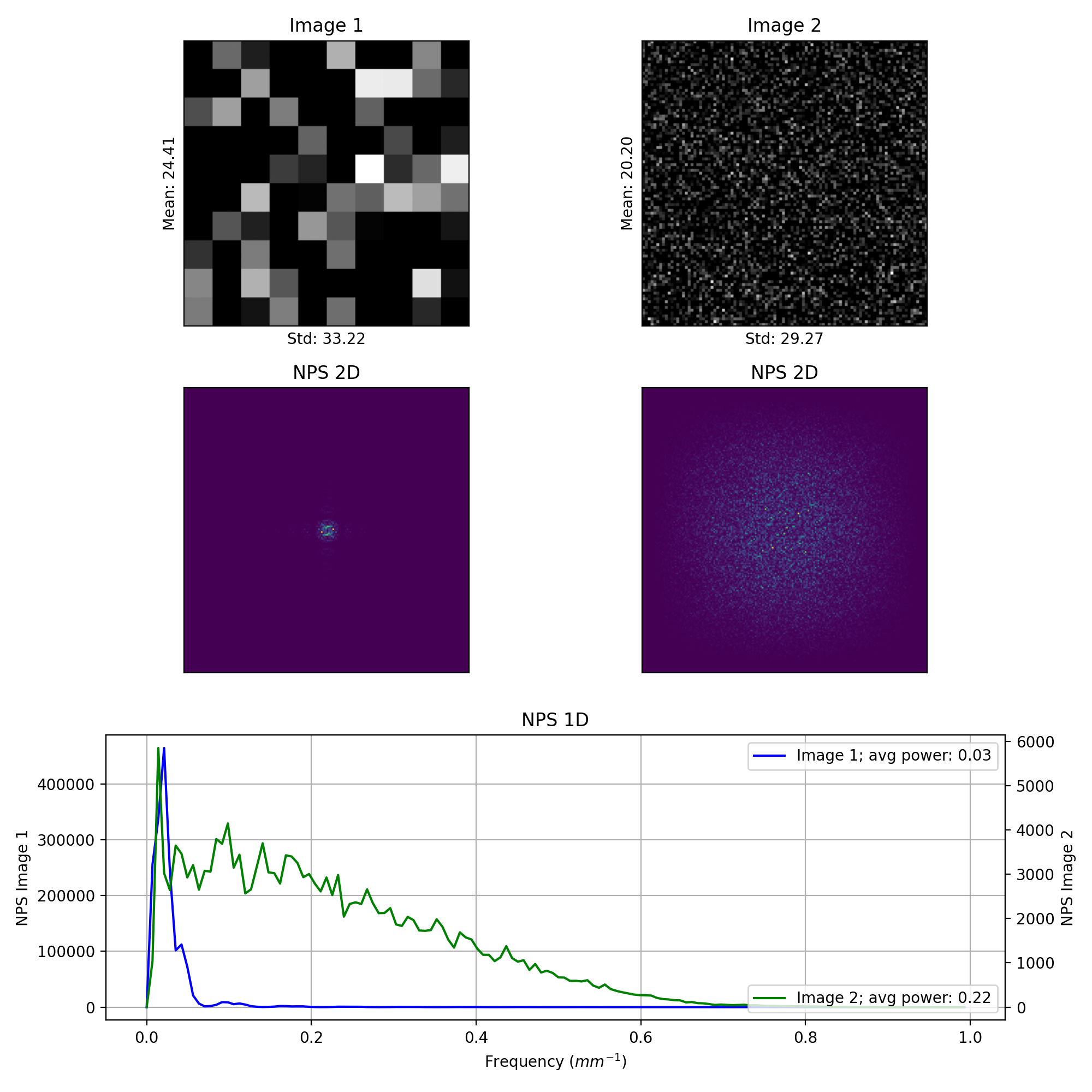
Let’s create a synthetic image and calculate the noise power spectrum, showing how images even with the same standard deviation can have different noise power spectra.
import matplotlib.pyplot as plt
import numpy as np

from pylinac.core.nps import noise_power_spectrum_2d, noise_power_spectrum_1d, average_power

np.random.seed(123)


def generate_gaussian_noise_map(shape: (int, int), scale: int=10, intensity: float=0.5):
    """Generate a Gaussian noise map with varying intensities (clumps).

    Parameters:
    - shape: Shape of the noise map (height, width).
    - scale: Scale of the Gaussian clumps.
    - intensity: Intensity of the noise.

    Returns:
    - Gaussian noise map as a NumPy array.
    """
    # Create low-resolution noise
    low_res_shape = (shape[0] // scale, shape[1] // scale)
    low_res_noise = np.random.normal(loc=0, scale=intensity, size=low_res_shape)

    # Upscale the noise to the original resolution
    noise_map = np.kron(low_res_noise, np.ones((scale, scale)))

    # Ensure the noise map matches the exact original shape, trimming if necessary
    noise_map = noise_map[:shape[0], :shape[1]]

    return noise_map


def apply_noise_clumps(image: np.ndarray, noise_map: np.ndarray) -> np.ndarray:
    """Apply a Gaussian noise map to an image.

    Parameters:
    - image: Original image as a NumPy array.
    - noise_map: Gaussian noise map.

    Returns:
    - Noisy image as a NumPy array.
    """
    noisy_image = image + noise_map
    dtype_min, dtype_max = np.iinfo(image.dtype).min, np.iinfo(image.dtype).max
    noisy_image = np.clip(noisy_image, dtype_min, dtype_max)

    return noisy_image

def generate_noisy_image(shape: (int, int), scale: int=10, intensity: float=0.5, dtype: np.dtype = np.uint16) -> np.ndarray:
    """Generate a noisy image with Gaussian clumps.

    Parameters:
    - image: Original image as a NumPy array.
    - scale: Scale of the Gaussian clumps.
    - intensity: Intensity of the noise.

    Returns:
    - Noisy image as a NumPy array.
    """
    latent = np.zeros(shape, dtype=dtype)
    noise_map = generate_gaussian_noise_map(latent.shape, scale, intensity)
    noisy_image = apply_noise_clumps(latent, noise_map)
    return noisy_image


img1 = generate_noisy_image(shape=(200, 200), scale=20, intensity=50, dtype=np.uint8)
img2 = generate_noisy_image(shape=(200, 200), scale=2, intensity=50, dtype=np.uint8)

# 2D power spectrum
# we use pixel size of 1 for simplicity
nps2d_1 = noise_power_spectrum_2d(pixel_size=1, rois=[img1])
nps2d_2 = noise_power_spectrum_2d(pixel_size=1, rois=[img2])

# 1D power spectrum
nps1d_1 = noise_power_spectrum_1d(spectrum_2d=nps2d_1)
nps1d_2 = noise_power_spectrum_1d(spectrum_2d=nps2d_2)

# plot the two images, their 2D power spectra, and a combined 1d power spectra plot
fig = plt.figure(figsize=(10, 10))
img1_ax = plt.subplot2grid((3, 2), (0, 0), fig=fig)
img1_ax.imshow(img1, cmap='gray')
img1_ax.set_title('Image 1')
img1_ax.set_xlabel(f'Std: {img1.std():.2f}')
img1_ax.set_ylabel(f'Mean: {img1.mean():.2f}')

img2_ax = plt.subplot2grid((3, 2), (0, 1))
img2_ax.imshow(img2, cmap='gray')
img2_ax.set_title('Image 2')
img2_ax.set_xlabel(f'Std: {img2.std():.2f}')
img2_ax.set_ylabel(f'Mean: {img2.mean():.2f}')

nps2d_1_ax = plt.subplot2grid((3, 2), (1, 0))
nps2d_1_ax.imshow(nps2d_1, cmap='viridis')
nps2d_1_ax.set_title('NPS 2D')

nps2d_2_ax = plt.subplot2grid((3, 2), (1, 1))
nps2d_2_ax.imshow(nps2d_2, cmap='viridis')
nps2d_2_ax.set_title('NPS 2D')

# turn off ticks
for ax in [img1_ax, img2_ax, nps2d_1_ax, nps2d_2_ax]:
    ax.set_xticks([])
    ax.set_yticks([])

x_vals = np.arange(len(nps1d_1))/len(nps1d_1)
nps1d_ax = plt.subplot2grid((3, 2), (2, 0), colspan=2)
nps1d_ax.plot(x_vals, nps1d_1, label=f'Image 1; avg power: {average_power(nps1d_1):.2f}', color='b')
nps1d_ax2 = nps1d_ax.twinx()
nps1d_ax2.plot(x_vals, nps1d_2, label=f'Image 2; avg power: {average_power(nps1d_2):.2f}', color='g')
nps1d_ax.set_title('NPS 1D')
nps1d_ax.set_xlabel('Frequency ($mm^{-1}$)')
nps1d_ax.set_ylabel('NPS Image 1')
nps1d_ax.grid(True)
nps1d_ax2.set_ylabel('NPS Image 2')
nps1d_ax.legend(loc='upper right')
nps1d_ax2.legend(loc='lower right')

plt.tight_layout()
plt.show()
(Source code, png, hires.png, pdf)
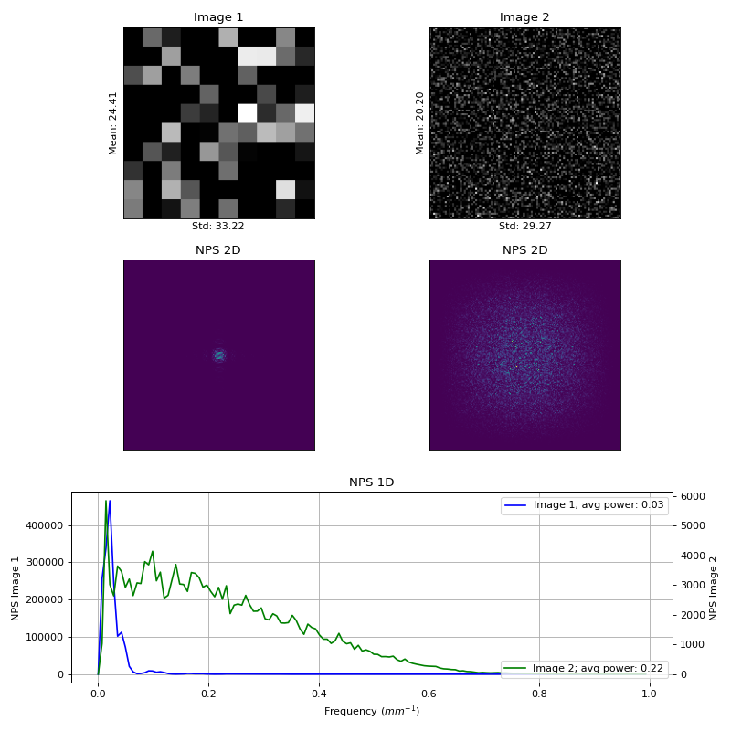
Even with roughly the same mean and standard deviation, the noise power spectrum is vastly different.
Note
The images are the same size in pixels. This image generator is a simplistic approach to generating synthetic CT images, but is useful for demonstrating the noise power spectrum.
References
API
- pylinac.core.nps.noise_power_spectrum_2d(pixel_size: float, rois: Iterable[ndarray]) ndarray[source]
Calculate the noise power spectrum in 2D and 1D for a set of square ROIs.
Based on ICRU 87, equation 11.1 and 11.2. Calculates the 2D FFT of each ROI, then averages the FFTs. FFTs are shifted so that the zero frequency is in the center and then radially averaged
Notes
The ROIs should be 2D and square (i.e. not a rectangle, circle, etc). The smallest dimension of the ROIs will be used. I.e. the ROIs can vary in size, but only the smallest dimension will be used. In practice, ROIs can sometimes vary depending on how they are extracted from an image (at least in pylinac). Sometimes the ROI may be 32 pixels wide and 30 pixels tall, for instance. In this case, the 30x30 subset of the ROI will be used.
Parameters
- pixel_sizefloat
The size of each pixel in mm.
- roislist of ndarray
A list of the ROIs to calculate the NPS over. Each ROI should be a 2D array.
Returns
- nps2dndarray
The 2D noise power spectrum.
References
- pylinac.core.nps.noise_power_spectrum_1d(spectrum_2d: ndarray) ndarray[source]
Calculate the 1D noise power spectrum from a 2D spectrum.
Parameters
- spectrum_2dndarray
The 2D noise power spectrum.
Returns
- ndarray
The 1D noise power spectrum.
- pylinac.core.nps.average_power(nps1d: ndarray) float[source]
Average power given a 1D spectra.
Parameters
- nps1dsequence of ndarray
The 1D noise power spectra to average.
Returns
- float
The average noise power spectrum value
- pylinac.core.nps.max_frequency(nps1d: ndarray) float[source]
Determine the maximum frequency of the NPS given a 1D spectrum.
- pylinac.core.nps.plot_nps1d(nps1d: ndarray, ax: Axis | None = None) Axis[source]
Plot the 1D noise power spectrum.
This will plot the power spectrum as a function of frequency. We also need to remove frequencies above the Nyquist frequency.
Parameters
- nps1dndarray
The 1D noise power spectrum.
- axmatplotlib.axis.Axis, optional
The axis to plot on. If None, a new figure will be created.
Returns
- matplotlib.axis.Axis
The axis the plot was created on.