VMAT#

Overview#

The VMAT module consists of the class VMAT, which is capable of loading an EPID DICOM Open field image and MLC field image and analyzing the images according to the Varian RapidArc QA tests and procedures, specifically the Dose-Rate & Gantry-Speed (DRGS) and Dose-Rate & MLC speed (DRMLC) tests.

Features:

Do both tests - Pylinac can handle either DRGS or DRMLC tests.
Automatic offset correction - Older VMAT tests had the ROIs offset, newer ones are centered. No worries, pylinac finds the ROIs automatically.
Automatic open/DMLC identification - Pass in both images–don’t worry about naming. Pylinac will automatically identify the right images.

Note

There are two classes in the VMAT module: DRGS and DRMLC. Each have the exact same methods. Anytime one class is used here as an example, the other class can be used the same way.

Running the Demos#

For this example we will use the DRGS class:

from pylinac import DRGS
DRGS.run_demo()

(Source code, png, hires.png, pdf)

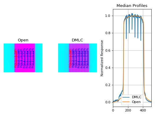
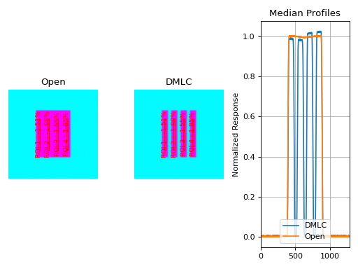
Results will be printed to the console and a figure showing both the Open field and MLC field image will pop up:

Dose Rate & Gantry Speed
Test Results (Tol. +/-1.5%): PASS
Max Deviation: 1.01%
Absolute Mean Deviation: 0.459%

Image Acquisition#

If you want to perform these specific QA tests, you’ll need DICOM plan files that control the linac precisely to deliver the test fields. These can be downloaded from my.varian.com. Once logged in, search for RapidArc and you should see two items called “RapidArc QA Test Procedures and Files for TrueBeam”; there will be a corresponding one for C-Series. Use the RT Plan files and follow the instructions, not including the assessment procedure, which is the point of this module. Save & move the VMAT images to a place you can use pylinac.

Typical Use#

The VMAT QA analysis follows what is specified in the Varian RapidArc QA tests and assumes your tests will run the exact same way. Import the appropriate class:

from pylinac import DRGS, DRMLC

The minimum needed to get going is to:

Load images – Loading the EPID DICOM images into your VMAT class object can be done by passing the file paths, passing a ZIP archive, or passing a URL:

open_img = "C:/QA Folder/VMAT/open_field.dcm"
dmlc_img = "C:/QA Folder/VMAT/dmlc_field.dcm"
mydrgs = DRGS(
    image_paths=(open_img, dmlc_img)
)  # use the DRMLC class the exact same way

# from zip
mydrmlc = DRMLC.from_zip(r"C:/path/to/zip.zip")

# from a URL
mydrgs = DRGS.from_url("http://myserver.org/vmat.zip")

Finally, if you don’t have any images, you can use the demo ones provided:

mydrgs = DRGS.from_demo_images()
mydrmlc = DRMLC.from_demo_images()

Analyze the images – Once the images are loaded, tell the class to analyze the images. See the Algorithm section for details on how this is done. Tolerance can also be passed and has a default value of 1.5%:
```
mydrgs.analyze(tolerance=1.5)
```
View/Save the results – The VMAT module can print out the summary of results to the console as well as draw a matplotlib image to show where the segments were placed and their values:
```
# print results to the console
print(mydrgs.results())
# view analyzed images
mydrgs.plot_analyzed_image()
```
(Source code, png, hires.png, pdf)

PDF reports can also be generated:
```
myvmat.publish_pdf("drgs.pdf")
```

Customizing the analysis#

You can alter both the segment size and segment positions as desired.

To change the segment size:

drgs = DRGS.from_demo_image()
drgs.analyze(
    ..., segment_size_mm=(10, 150)
)  # ROI segments will now be 10mm wide by 150mm tall
# same story for DRMLC

To change the x-positions of the ROI segments or change the number of ROI, use a custom ROI config dictionary and pass it to the analyze method.

from pylinac import DRGS, DRMLC

# note the keys are the names of the ROIs and can be anything you like
custom_roi_config = {
    "200 MU/min": {"offset_mm": -100},
    "300 MU/min": {"offset_mm": -80},
}  # add more as needed

my_drgs = DRGS(...)  # works the same way for DRMLC
my_drgs.analyze(..., roi_config=custom_roi_config)

(Source code, png, hires.png, pdf)

Accessing Data#

Changed in version 3.0.

Using the VMAT module in your own scripts? While the analysis results can be printed out, if you intend on using them elsewhere (e.g. in an API), they can be accessed the easiest by using the results_data() method which returns a VMATResult instance.

Note

While the pylinac tooling may change under the hood, this object should remain largely the same and/or expand. Thus, using this is more stable than accessing attrs directly.

Continuing from above:

data = my_drmlc.results_data()
data.test_type
data.passed
# and more

# return as a dict
data_dict = my_drmlc.results_data(as_dict=True)
data_dict["test_type"]
...

Algorithm#

The VMAT analysis algorithm is based on the Varian RapidArc QA Test Procedures for C-Series and Truebeam. Two tests (besides Picket Fence, which has its own module) are specified. Each test takes 10x0.5cm samples, each corresponding to a distinct section of radiation. A corrected reading of each segment is made, defined as: \(M_{corr}(x) = \frac{M_{DRGS}(x)}{M_{open}(x)} * 100\). The reading deviation of each segment is calculated as: \(M_{deviation}(x) = \frac{M_{corr}(x)}{\bar{M_{corr}}} * 100 - 100\), where \(\bar{M_{corr}}\) is the average of all segments.

The algorithm works like such:

Allowances

The images can be acquired at any SID.
The images can be acquired with any EPID (aS500, aS1000, aS1200).

Restrictions

Warning

Analysis can fail or give unreliable results if any Restriction is violated.

The tests must be delivered using the DICOM RT plan files provided by Varian which follow the test layout of Ling et al.
The images must be acquired with the EPID.

Pre-Analysis

Determine image scaling – Segment determination is based on offsets from the center pixel of the image. However, some physicists use 150 cm SID and others use 100 cm, and others can use a clinical setting that may be different than either of those. To account for this, the SID is determined and then scaling factors are determined to be able to perform properly-sized segment analysis.

Analysis

Note

Calculations tend to be lazy, computed only on demand. This represents a nominal analysis where all calculations are performed.

Calculate sample boundaries – The Segment x-positions are based on offsets from the center of the FWHM of the detected field. This allows for old and new style tests that have an x-offset from each other. These values are then scaled with the image scaling factor determined above.
Calculate the corrected reading – For each segment, the mean pixel value is determined for both the open and DMLC image. These values are used to determine the corrected reading: \(M_{corr}\).
Calculate sample and segment ratios – The sample values of the DMLC field are divided by their corresponding open field values.
Calculate segment deviations – Segment deviation is then calculated once all the corrected readings are determined. The average absolute deviation is also calculated.

Post-Analysis

Test if segments pass tolerance – Each segment is checked to see if it was within the specified tolerance. If any samples fail, the whole test is considered failing.

Benchmarking the Algorithm#

With the image generator module we can create test images to test the VMAT algorithm on known results. This is useful to isolate what is or isn’t working if the algorithm doesn’t work on a given image and when commissioning pylinac.

Note

The below examples are for the DRMLC test but can equally be applied to the DRGS tests as well.

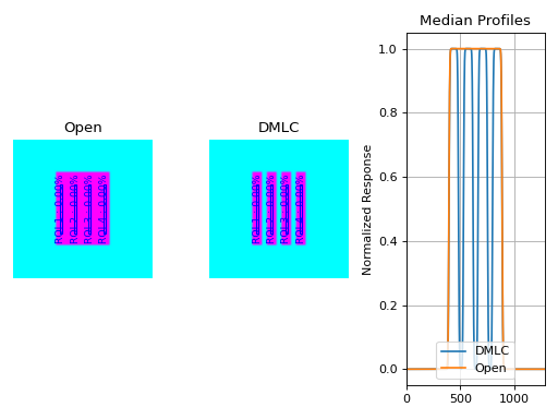
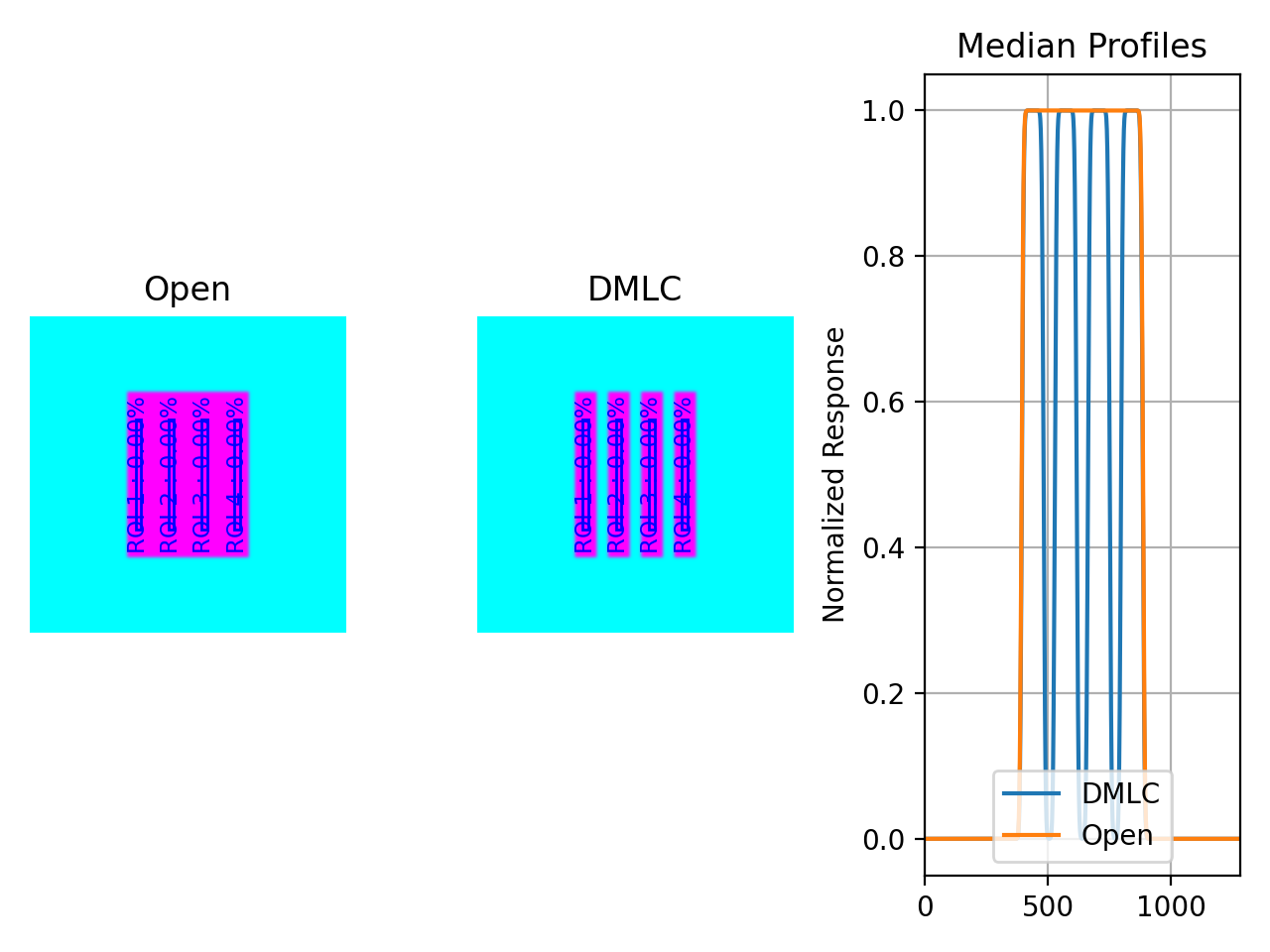
Perfect Fields#

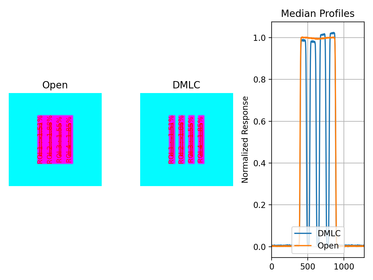
In this example, we generate a perfectly flat set of images and analyze them.

import pylinac
from pylinac.core.image_generator import GaussianFilterLayer, PerfectFieldLayer, AS1200Image

# open image
open_path = 'perfect_open_drmlc.dcm'
as1200 = AS1200Image()
as1200.add_layer(PerfectFieldLayer(field_size_mm=(150, 85), cax_offset_mm=(0, 0)))
as1200.add_layer(GaussianFilterLayer(sigma_mm=2))
as1200.generate_dicom(file_out_name=open_path)

# DMLC image
dmlc_path = 'perfect_dmlc_drmlc.dcm'
as1200 = AS1200Image()
for offset in (-45, -15, 15, 45):
    as1200.add_layer(PerfectFieldLayer((150, 19.5), cax_offset_mm=(0, offset)))
as1200.add_layer(GaussianFilterLayer(sigma_mm=2))
as1200.generate_dicom(file_out_name=dmlc_path)

# analyze it
vmat = pylinac.DRMLC(image_paths=(open_path, dmlc_path))
vmat.analyze()
print(vmat.results())
vmat.plot_analyzed_image()

(Source code, png, hires.png, pdf)

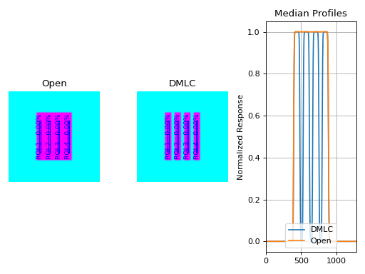
with output:

Dose Rate & MLC Speed
Test Results (Tol. +/-1.5%): PASS
Max Deviation: 0.0%
Absolute Mean Deviation: 0.0%

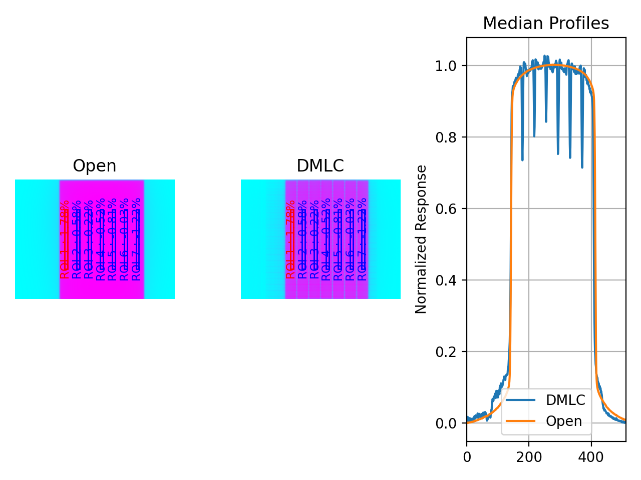
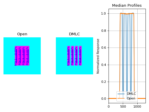
Noisy, Realistic#

We now add a horn effect and random noise to the data:

import pylinac
from pylinac.core.image_generator import GaussianFilterLayer, FilteredFieldLayer, AS1200Image, RandomNoiseLayer

# open image
open_path = 'noisy_open_drmlc.dcm'
as1200 = AS1200Image()
as1200.add_layer(FilteredFieldLayer(field_size_mm=(150, 85), cax_offset_mm=(0, 0)))
as1200.add_layer(GaussianFilterLayer(sigma_mm=2))
as1200.add_layer(RandomNoiseLayer(sigma=0.03))
as1200.generate_dicom(file_out_name=open_path)

# DMLC image
dmlc_path = 'noisy_dmlc_drmlc.dcm'
as1200 = AS1200Image()
for offset in (-45, -15, 15, 45):
    as1200.add_layer(FilteredFieldLayer((150, 19.5), cax_offset_mm=(0, offset)))
as1200.add_layer(GaussianFilterLayer(sigma_mm=2))
as1200.add_layer(RandomNoiseLayer(sigma=0.03))
as1200.generate_dicom(file_out_name=dmlc_path)

# analyze it
vmat = pylinac.DRMLC(image_paths=(open_path, dmlc_path))
vmat.analyze()
print(vmat.results())
vmat.plot_analyzed_image()

(Source code, png, hires.png, pdf)

with output:

Dose Rate & MLC Speed
Test Results (Tol. +/-1.5%): PASS
Max Deviation: 0.0332%
Absolute Mean Deviation: 0.0257%

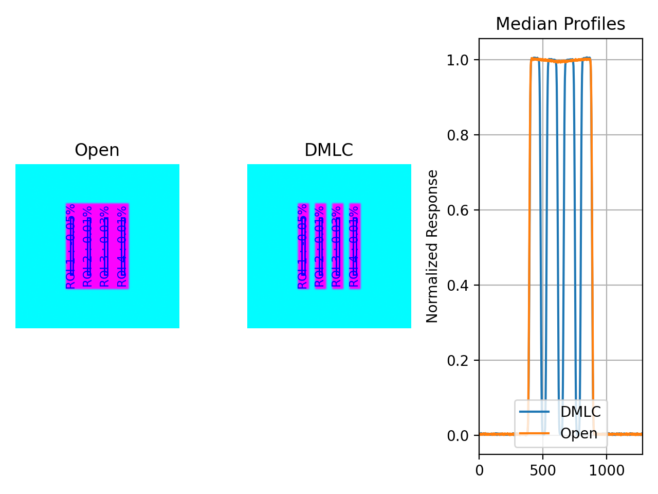
Erroneous data#

Let’s now get devious and randomly adjust the height of each ROI (effectively changing the apparent MLC speed):

Note

Due to the purposely random nature shown below, this exact result is likely not reproducible, nor was it intended to be. To get reproducible behavior, use numpy with a seed value.

import random

import pylinac
from pylinac.core.image_generator import GaussianFilterLayer, FilteredFieldLayer, AS1200Image, RandomNoiseLayer

# open image
open_path = 'noisy_open_drmlc.dcm'
as1200 = AS1200Image()
as1200.add_layer(FilteredFieldLayer(field_size_mm=(150, 85), cax_offset_mm=(0, 0)))
as1200.add_layer(GaussianFilterLayer(sigma_mm=2))
as1200.add_layer(RandomNoiseLayer(sigma=0.03))
as1200.generate_dicom(file_out_name=open_path)

# DMLC image
dmlc_path = 'noisy_dmlc_drmlc.dcm'
as1200 = AS1200Image()
for offset in (-45, -15, 15, 45):
    as1200.add_layer(FilteredFieldLayer((150, 19.5), cax_offset_mm=(0, offset), alpha=random.uniform(0.93, 1)))
as1200.add_layer(GaussianFilterLayer(sigma_mm=2))
as1200.add_layer(RandomNoiseLayer(sigma=0.04))
as1200.generate_dicom(file_out_name=dmlc_path)

# analyze it
vmat = pylinac.DRMLC(image_paths=(open_path, dmlc_path))
vmat.analyze()
print(vmat.results())
vmat.plot_analyzed_image()

(Source code, png, hires.png, pdf)

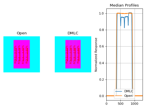
with an output of:

Dose Rate & MLC Speed
Test Results (Tol. +/-1.5%): FAIL
Max Deviation: 2.12%
Absolute Mean Deviation: 1.13%

Comparing to other programs#

Note

The DRGS pattern is used as an example but the same concepts applies to both DRGS and DRMLC.

A common question is how results should be compared to other programs. While the answer will depend on several factors, we can make some general observations here.

Ensure the ROI sizes are similar - Different programs may have different defaults for the ROI size. Varian suggests a 5x100mm rectangular ROI, although this seems arbitrarily small in our opinion. In any event, to match Varian’s suggestion, the pylinac default segment ROI size is 5x100mm
DICOM images may have different reconstruction algorithms - Pylinac’s DICOM image loading algorithm can be read here: Pixel Data & Inversion. It tries to use as many tags as it can to reconstruct the correct pixel values. However, this behavior does not appear consistent across all programs. E.g. if tags are not considered when loading images, the resulting pixels (and thus ratio) may not match an image that did use tags.

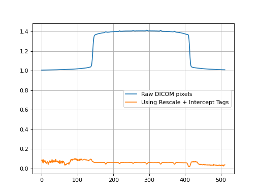
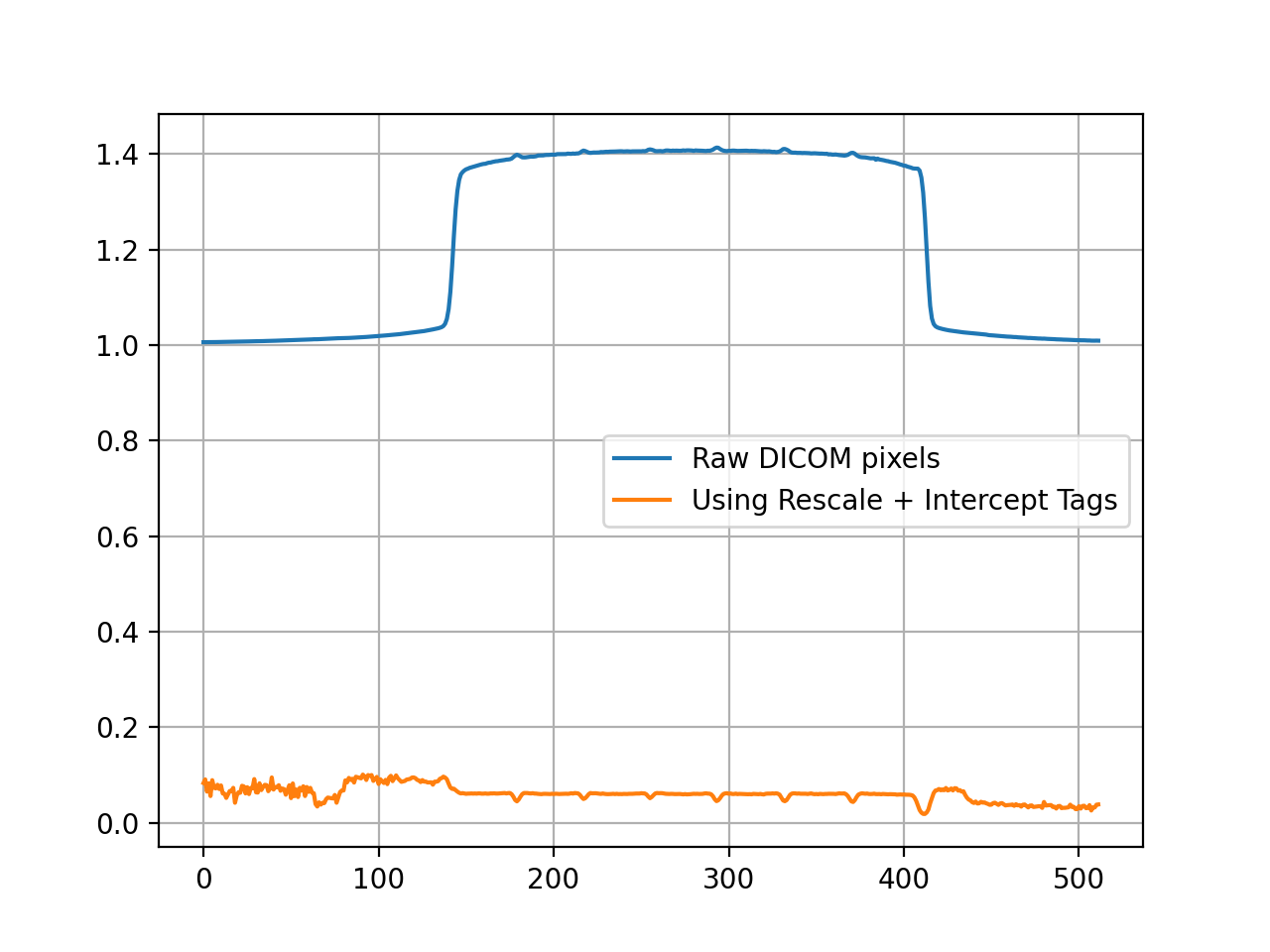
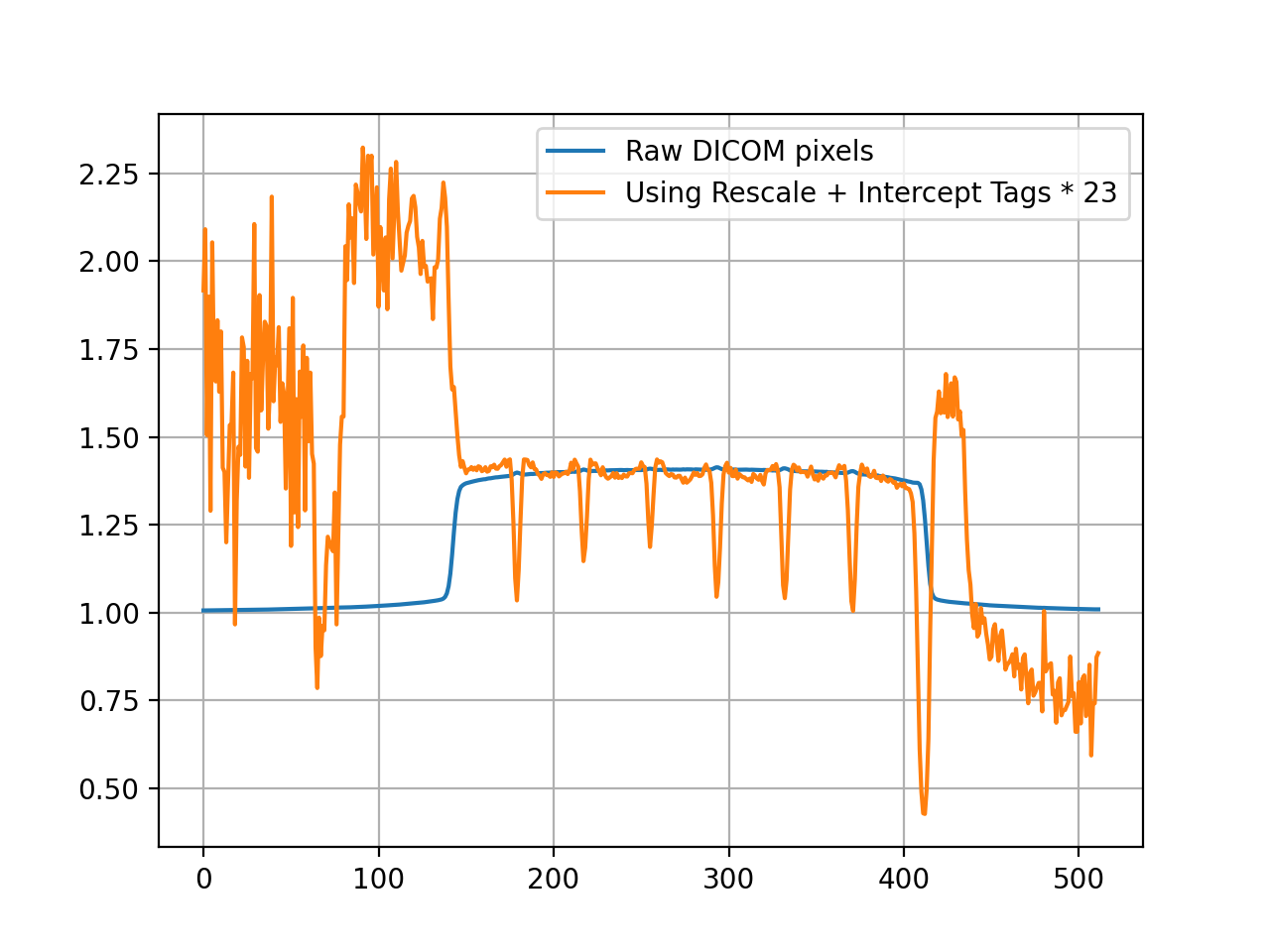
Take for instance the below example comparing “raw” pixel values to using the Tag-corrected version:
```
from matplotlib import pyplot as plt
import pydicom

from pylinac import image
from pylinac.core.io import retrieve_demo_file, TemporaryZipDirectory

demo_zip = retrieve_demo_file('drgs.zip')
with TemporaryZipDirectory(demo_zip) as tmpzip:
    image_files = image.retrieve_image_files(tmpzip)

    # read the values "raw"
    dmlc_raw = pydicom.read_file(image_files[0])
    open_raw = pydicom.read_file(image_files[1])
    raw = dmlc_raw.pixel_array / open_raw.pixel_array

    # Tag-correct the values
    img_dmlc = image.load(image_files[0])
    img_open = image.load(image_files[1])
    corrected = img_dmlc.array / img_open.array

plt.plot(raw[200, :], label="Raw DICOM pixels")
plt.plot(corrected[200, :], label="Using Rescale + Intercept Tags")
plt.legend()
plt.grid(True)
plt.show()
```
(Source code, png, hires.png, pdf)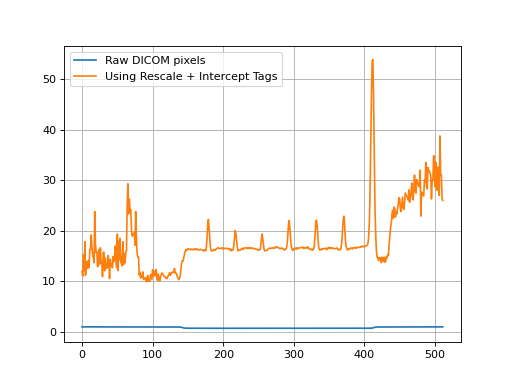

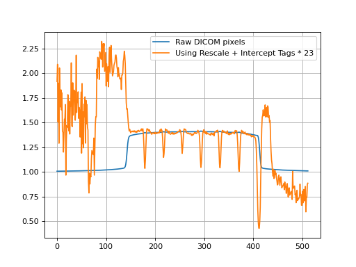
We can also scale the tag-corrected value for the purpose of comparing relative responses:

(Source code, png, hires.png, pdf)

The point of the second plot is to show what the ratio of each ROI looks like between the normalizations. Inspecting the left-most ROI, we see that the raw pixel normalization is lower than the average ROI response, whereas with the tag-corrected implementation, it’s actually higher. When evaluating the ROI results of pylinac vs other programs this explains why the left-most ROI (which is used simply as an example) has a positive deviation whereas other programs may have a negative deviation.

This behavior can change depending on the tags available in the DICOM file. Newer DICOMs also have a “sign” tag to correct for inversion of pixel data. Why this difference can be problematic is that the ratio of the open to DMLC image depends on the initial pixel value.

Currently, this is a philosophical difference between programs that don’t use DICOM tags and those that do, like pylinac. If the goal is to switch from another program to pylinac, the standard approach of measuring with both algorithms to establish a baseline of differences is recommended, just as you might when switching from a water tank measurement to an array-based measurement scheme.

Comparison to Doselab#

New in version 3.13.

All that being said, if the goal is to match another program (specifically, Doselab, although this might apply to others) use the following:

from pylinac import DRMLC

drmlc = DRMLC(..., raw_pixels=True, ground=False, check_inversion=False)
...

This will skip the checking of DICOM tags for correcting the pixel values as well as other manipulations normally applied.

Here’s a table comparing the results of the DRMLC demo dataset with different variations:

	Max R_dev	ROI 1 R_dev	ROI 2 R_dev	ROI 3 R_dev	ROI 4 R_dev
Doselab (normalized)		0.995	1.005	1.006	0.994
Doselab (as % from unity)	0.60%	-0.50%	0.50%	0.60%	-0.60%
Pylinac (raw=True, ground=False, inversion=False)	0.56%	-0.54%	0.53%	0.56%	-0.55%
Pylinac (default)	0.89%	-0.68%	0.89%	-0.10%	-0.11%
Pylinac (raw=False, ground=False, inversion=False)	0.90%	-0.68%	0.90%	-0.08%	-0.12%

The Doselab and pylinac results are very similar when the raw pixels are used. The default settings and the analysis without any extra manipulations are also extremely similar.

Note

For historical continuity, the manipulations are set to True. If you are just starting to use Pylinac, it is recommended to use the settings of the last row. However, it is unlikely to make a significant difference.

API Documentation#

Main classes#

These are the classes a typical user may interface with.

class pylinac.vmat.DRGS(image_paths: Sequence[str | BinaryIO | Path], ground=True, check_inversion=True, **kwargs)[source]#

Bases: VMATBase

Class representing a Dose-Rate, Gantry-speed VMAT test. Will accept, analyze, and return the results.

Parameters#

image_pathsiterable (list, tuple, etc): A sequence of paths to the image files.
kwargs: Passed to the image loading function. See load().

static run_demo()[source]#: Run the demo for the Dose Rate & Gantry Speed test.

analyze(tolerance: float | int = 1.5, segment_size_mm: tuple = (5, 100), roi_config: dict | None = None)#

Analyze the open and DMLC field VMAT images, according to 1 of 2 possible tests.

Parameters#

tolerancefloat, int, optional: The tolerance of the sample deviations in percent. Default is 1.5. Must be between 0 and 8.
segment_size_mmtuple(int, int): The (width, height) of the ROI segments in mm.
roi_configdict: A dict of the ROI settings. The keys are the names of the ROIs and each value is a dict containing the offset in mm ‘offset_mm’.

property avg_abs_r_deviation: float#: Return the average of the absolute R_deviation values.

property avg_r_deviation: float#: Return the average of the R_deviation values, including the sign.

classmethod from_demo_images(**kwargs)#: Construct a VMAT instance using the demo images.

classmethod from_url(url: str)#

Load a ZIP archive from a URL. Must follow the naming convention.

Parameters#

urlstr: Must point to a valid URL that is a ZIP archive of two VMAT images.

classmethod from_zip(path: str | Path, **kwargs)#

Load VMAT images from a ZIP file that contains both images. Must follow the naming convention.

Parameters#

pathstr: Path to the ZIP archive which holds the VMAT image files.
kwargs: Passed to the constructor.

property max_r_deviation: float#: Return the value of the maximum R_deviation segment.

plot_analyzed_image(show: bool = True, show_text: bool = True, **plt_kwargs: dict)#

Plot the analyzed images. Shows the open and dmlc images with the segments drawn; also plots the median profiles of the two images for visual comparison.

Parameters#

showbool: Whether to actually show the image.
show_textbool: Whether to show the ROI names on the image.
plt_kwargsdict: Keyword args passed to the plt.subplots() method. Allows one to set things like figure size.

publish_pdf(filename: str, notes: str = None, open_file: bool = False, metadata: dict | None = None, logo: Path | str | None = None)#

Publish (print) a PDF containing the analysis, images, and quantitative results.

Parameters#

filename(str, file-like object}: The file to write the results to.
notesstr, list of strings: Text; if str, prints single line. If list of strings, each list item is printed on its own line.
open_filebool: Whether to open the file using the default program after creation.
metadatadict: Extra data to be passed and shown in the PDF. The key and value will be shown with a colon. E.g. passing {‘Author’: ‘James’, ‘Unit’: ‘TrueBeam’} would result in text in the PDF like: ————– Author: James Unit: TrueBeam ————–
logo: Path, str: A custom logo to use in the PDF report. If nothing is passed, the default pylinac logo is used.

property r_devs: ndarray#: Return the deviations of all segments as an array.

results() → str#

A string of the summary of the analysis results.

Returns#

str: The results string showing the overall result and deviation statistics by segment.

results_data(as_dict: bool = False, as_json: bool = False) → T | dict | str#

Present the results data and metadata as a dataclass, dict, or tuple. The default return type is a dataclass.

Parameters#

as_dictbool: If True, return the results as a dictionary.
as_jsonbool: If True, return the results as a JSON string. Cannot be True if as_dict is True.

class pylinac.vmat.DRMLC(image_paths: Sequence[str | BinaryIO | Path], ground=True, check_inversion=True, **kwargs)[source]#

Bases: VMATBase

Class representing a Dose-Rate, MLC speed VMAT test. Will accept, analyze, and return the results.

Parameters#

image_pathsiterable (list, tuple, etc): A sequence of paths to the image files.
kwargs: Passed to the image loading function. See load().

analyze(tolerance: float | int = 1.5, segment_size_mm: tuple = (5, 100), roi_config: dict | None = None)#

Analyze the open and DMLC field VMAT images, according to 1 of 2 possible tests.

Parameters#

tolerancefloat, int, optional: The tolerance of the sample deviations in percent. Default is 1.5. Must be between 0 and 8.
segment_size_mmtuple(int, int): The (width, height) of the ROI segments in mm.
roi_configdict: A dict of the ROI settings. The keys are the names of the ROIs and each value is a dict containing the offset in mm ‘offset_mm’.

property avg_abs_r_deviation: float#: Return the average of the absolute R_deviation values.

property avg_r_deviation: float#: Return the average of the R_deviation values, including the sign.

classmethod from_demo_images(**kwargs)#: Construct a VMAT instance using the demo images.

classmethod from_url(url: str)#

Load a ZIP archive from a URL. Must follow the naming convention.

Parameters#

urlstr: Must point to a valid URL that is a ZIP archive of two VMAT images.

classmethod from_zip(path: str | Path, **kwargs)#

Load VMAT images from a ZIP file that contains both images. Must follow the naming convention.

Parameters#

pathstr: Path to the ZIP archive which holds the VMAT image files.
kwargs: Passed to the constructor.

property max_r_deviation: float#: Return the value of the maximum R_deviation segment.

plot_analyzed_image(show: bool = True, show_text: bool = True, **plt_kwargs: dict)#

Plot the analyzed images. Shows the open and dmlc images with the segments drawn; also plots the median profiles of the two images for visual comparison.

Parameters#

showbool: Whether to actually show the image.
show_textbool: Whether to show the ROI names on the image.
plt_kwargsdict: Keyword args passed to the plt.subplots() method. Allows one to set things like figure size.

publish_pdf(filename: str, notes: str = None, open_file: bool = False, metadata: dict | None = None, logo: Path | str | None = None)#

Publish (print) a PDF containing the analysis, images, and quantitative results.

Parameters#

filename(str, file-like object}: The file to write the results to.
notesstr, list of strings: Text; if str, prints single line. If list of strings, each list item is printed on its own line.
open_filebool: Whether to open the file using the default program after creation.
metadatadict: Extra data to be passed and shown in the PDF. The key and value will be shown with a colon. E.g. passing {‘Author’: ‘James’, ‘Unit’: ‘TrueBeam’} would result in text in the PDF like: ————– Author: James Unit: TrueBeam ————–
logo: Path, str: A custom logo to use in the PDF report. If nothing is passed, the default pylinac logo is used.

property r_devs: ndarray#: Return the deviations of all segments as an array.

results() → str#

A string of the summary of the analysis results.

Returns#

str: The results string showing the overall result and deviation statistics by segment.

results_data(as_dict: bool = False, as_json: bool = False) → T | dict | str#

Present the results data and metadata as a dataclass, dict, or tuple. The default return type is a dataclass.

Parameters#

as_dictbool: If True, return the results as a dictionary.
as_jsonbool: If True, return the results as a JSON string. Cannot be True if as_dict is True.

static run_demo()[source]#: Run the demo for the MLC leaf speed test.

class pylinac.vmat.VMATResult(*, pylinac_version: str = '3.22.0', date_of_analysis: datetime = None, test_type: str, tolerance_percent: float, max_deviation_percent: float, abs_mean_deviation: float, passed: bool, segment_data: Iterable[SegmentResult], named_segment_data: dict[str, SegmentResult])[source]#

Bases: ResultBase

This class should not be called directly. It is returned by the results_data() method. It is a dataclass under the hood and thus comes with all the dunder magic.

Use the following attributes as normal class attributes.

Create a new model by parsing and validating input data from keyword arguments.

Raises [ValidationError][pydantic_core.ValidationError] if the input data cannot be validated to form a valid model.

self is explicitly positional-only to allow self as a field name.

test_type: str#

tolerance_percent: float#

max_deviation_percent: float#

abs_mean_deviation: float#

passed: bool#

segment_data: Iterable[SegmentResult]#

named_segment_data: dict[str, SegmentResult]#

model_computed_fields: ClassVar[dict[str, ComputedFieldInfo]] = {}#: A dictionary of computed field names and their corresponding ComputedFieldInfo objects.

model_config: ClassVar[ConfigDict] = {'arbitrary_types_allowed': True}#: Configuration for the model, should be a dictionary conforming to [ConfigDict][pydantic.config.ConfigDict].

model_fields: ClassVar[dict[str, FieldInfo]] = {'abs_mean_deviation': FieldInfo(annotation=float, required=True), 'date_of_analysis': FieldInfo(annotation=datetime, required=False, default_factory=builtin_function_or_method), 'max_deviation_percent': FieldInfo(annotation=float, required=True), 'named_segment_data': FieldInfo(annotation=dict[str, SegmentResult], required=True), 'passed': FieldInfo(annotation=bool, required=True), 'pylinac_version': FieldInfo(annotation=str, required=False, default='3.22.0'), 'segment_data': FieldInfo(annotation=Iterable[SegmentResult], required=True), 'test_type': FieldInfo(annotation=str, required=True), 'tolerance_percent': FieldInfo(annotation=float, required=True)}#

Metadata about the fields defined on the model, mapping of field names to [FieldInfo][pydantic.fields.FieldInfo].

This replaces Model.__fields__ from Pydantic V1.

class pylinac.vmat.SegmentResult(*, passed: bool, x_position_mm: float, r_corr: float, r_dev: float, center_x_y: Point, stdev: float)[source]#

Bases: BaseModel

An individual segment/ROI result

Create a new model by parsing and validating input data from keyword arguments.

Raises [ValidationError][pydantic_core.ValidationError] if the input data cannot be validated to form a valid model.

self is explicitly positional-only to allow self as a field name.

model_config: ClassVar[ConfigDict] = {'arbitrary_types_allowed': True}#: Configuration for the model, should be a dictionary conforming to [ConfigDict][pydantic.config.ConfigDict].

passed: bool#

x_position_mm: float#

r_corr: float#

r_dev: float#

center_x_y: PointSerialized#

stdev: float#

model_computed_fields: ClassVar[dict[str, ComputedFieldInfo]] = {}#: A dictionary of computed field names and their corresponding ComputedFieldInfo objects.

model_fields: ClassVar[dict[str, FieldInfo]] = {'center_x_y': FieldInfo(annotation=Point, required=True, metadata=[PlainSerializer(func=<function to_json>, return_type=PydanticUndefined, when_used='always')]), 'passed': FieldInfo(annotation=bool, required=True), 'r_corr': FieldInfo(annotation=float, required=True), 'r_dev': FieldInfo(annotation=float, required=True), 'stdev': FieldInfo(annotation=float, required=True), 'x_position_mm': FieldInfo(annotation=float, required=True)}#

Metadata about the fields defined on the model, mapping of field names to [FieldInfo][pydantic.fields.FieldInfo].

This replaces Model.__fields__ from Pydantic V1.

Supporting Classes#

You generally won’t have to interface with these unless you’re doing advanced behavior.

class pylinac.vmat.VMATBase(image_paths: Sequence[str | BinaryIO | Path], ground=True, check_inversion=True, **kwargs)[source]#

Bases: ResultsDataMixin[VMATResult]

Parameters#

image_pathsiterable (list, tuple, etc): A sequence of paths to the image files.
kwargs: Passed to the image loading function. See load().

classmethod from_url(url: str)[source]#

Load a ZIP archive from a URL. Must follow the naming convention.

Parameters#

urlstr: Must point to a valid URL that is a ZIP archive of two VMAT images.

classmethod from_zip(path: str | Path, **kwargs)[source]#

Load VMAT images from a ZIP file that contains both images. Must follow the naming convention.

Parameters#

pathstr: Path to the ZIP archive which holds the VMAT image files.
kwargs: Passed to the constructor.

classmethod from_demo_images(**kwargs)[source]#: Construct a VMAT instance using the demo images.

analyze(tolerance: float | int = 1.5, segment_size_mm: tuple = (5, 100), roi_config: dict | None = None)[source]#

Analyze the open and DMLC field VMAT images, according to 1 of 2 possible tests.

Parameters#

tolerancefloat, int, optional: The tolerance of the sample deviations in percent. Default is 1.5. Must be between 0 and 8.
segment_size_mmtuple(int, int): The (width, height) of the ROI segments in mm.
roi_configdict: A dict of the ROI settings. The keys are the names of the ROIs and each value is a dict containing the offset in mm ‘offset_mm’.

results() → str[source]#

A string of the summary of the analysis results.

Returns#

str: The results string showing the overall result and deviation statistics by segment.

property r_devs: ndarray#: Return the deviations of all segments as an array.

property avg_abs_r_deviation: float#: Return the average of the absolute R_deviation values.

property avg_r_deviation: float#: Return the average of the R_deviation values, including the sign.

property max_r_deviation: float#: Return the value of the maximum R_deviation segment.

plot_analyzed_image(show: bool = True, show_text: bool = True, **plt_kwargs: dict)[source]#

Plot the analyzed images. Shows the open and dmlc images with the segments drawn; also plots the median profiles of the two images for visual comparison.

Parameters#

showbool: Whether to actually show the image.
show_textbool: Whether to show the ROI names on the image.
plt_kwargsdict: Keyword args passed to the plt.subplots() method. Allows one to set things like figure size.

publish_pdf(filename: str, notes: str = None, open_file: bool = False, metadata: dict | None = None, logo: Path | str | None = None)[source]#

Publish (print) a PDF containing the analysis, images, and quantitative results.

Parameters#

filename(str, file-like object}: The file to write the results to.
notesstr, list of strings: Text; if str, prints single line. If list of strings, each list item is printed on its own line.
open_filebool: Whether to open the file using the default program after creation.
metadatadict: Extra data to be passed and shown in the PDF. The key and value will be shown with a colon. E.g. passing {‘Author’: ‘James’, ‘Unit’: ‘TrueBeam’} would result in text in the PDF like: ————– Author: James Unit: TrueBeam ————–
logo: Path, str: A custom logo to use in the PDF report. If nothing is passed, the default pylinac logo is used.

results_data(as_dict: bool = False, as_json: bool = False) → T | dict | str#

Present the results data and metadata as a dataclass, dict, or tuple. The default return type is a dataclass.

Parameters#

as_dictbool: If True, return the results as a dictionary.
as_jsonbool: If True, return the results as a JSON string. Cannot be True if as_dict is True.

class pylinac.vmat.Segment(center_point: Point, open_image: DicomImage, dmlc_image: DicomImage, tolerance: float | int)[source]#

Bases: Rectangle

A class for holding and analyzing segment data of VMAT tests.

For VMAT tests, there are either 4 or 7 ‘segments’, which represents a section of the image that received radiation under the same conditions.

Attributes#

r_devfloat: The reading deviation (R_dev) from the average readings of all the segments. See documentation for equation info.

Parameters#

widthnumber: Width of the rectangle. Must be positive
heightnumber: Height of the rectangle. Must be positive.
centerPoint, iterable, optional: Center point of rectangle.
as_intbool: If False (default), inputs are left as-is. If True, all inputs are converted to integers.

property r_corr: float#: Return the ratio of the mean pixel values of DMLC/OPEN images.

property stdev: float#: Return the standard deviation of the segment.

property passed: bool#: Return whether the segment passed or failed.

get_bg_color() → str[source]#: Get the background color of the segment when plotted, based on the pass/fail status.

property area: float#: The area of the rectangle.

property bl_corner: Point#: The location of the bottom left corner.

property br_corner: Point#: The location of the bottom right corner.

plot2axes(axes: Axes, edgecolor: str = 'black', angle: float = 0.0, fill: bool = False, alpha: float = 1, facecolor: str = 'g', label=None, text: str = '', fontsize: str = 'medium', text_rotation: float = 0, **kwargs)#

Plot the Rectangle to the axes.

Parameters#

axesmatplotlib.axes.Axes: An MPL axes to plot to.
edgecolorstr: The color of the circle.
anglefloat: Angle of the rectangle.
fillbool: Whether to fill the rectangle with color or leave hollow.
text: str: If provided, plots the given text at the center. Useful for identifying ROIs on a plotted image apart.
fontsize: str: The size of the text, if provided. See https://matplotlib.org/stable/api/_as_gen/matplotlib.pyplot.text.html for options.
text_rotation: float: The rotation of the text in degrees.

property tl_corner: Point#: The location of the top left corner.

property tr_corner: Point#: The location of the top right corner.