Plan Generator¶

The plan generator is a tool for generating QA plans customized for user needs. It can create typical plans like picket fence, open fields, gantry speed, MLC speed, Winston-Lutz, dose rate constancy tests and more.

Warning

This tool is meant for research and QA activities. It is not meant for actual patient treatment or use. Do not use this in conjunction with a patient plan.

Warning

The module is still experimental. It will take a few releases to work out the kinks. It’s also primarily designed for Varian machines and the Eclipse TPS (the defaults are set for such a configuration).

Note

Units of parameters are always in mm and degrees unless otherwise specified. Parameter names are usually explicit for non-standard terms but are sometimes assumed for common terms/parameters.

Prerequisites¶

To use the plan generator a base RT Plan file (or dataset) is required from the machine and institution it will be generating for. This is easy to do in Eclipse (and likely other TPSs) by creating/using a QA patient and creating a simple plan on the machine of interest. The plan should have at least 1 field and the field must contain MLCs. The MLCs don’t have to do anything; it doesn’t need to be dynamic plan. The point is that a plan like this, regardless of what the MLCs are doing, simply contains the MLC setup information. In list form, the plan should:

Be based on a QA/research patient in your R&V (no real patients)
Have a field with MLCs (static or dynamic)
Be set to the machine of interest
Set the tolerance table to the desired table

Once the plan is created and saved, export it to a DICOM file. This file will be used as the base plan for the generator.

This entire process can be done in the Plan Parameters of Eclipse as shown below:

Use DICOM Import/Export to export the plan to a file.

Typical Use¶

Once a DICOM plan is generated and downloaded, it can be passed to the Plan Generator. The plan generator can then add QA fields into the plan.

from pylinac.plan_generator.dicom import PlanGenerator

rt_plan_file = r"C:\path\to\plan.dcm"
generator = PlanGenerator.from_rt_plan_file(
    rt_plan_file, plan_name="New QA Plan", plan_label="New QA"
)

# add a picket fence beam
generator.add_picketfence_beam(
    strip_width_mm=3,
    strip_positions_mm=(-100, -50, 20, 80),  # 4 pickets
    mu=100,
    beam_name="PF 3mm",
    y1=-150,
    y2=150,  # set y-jaws so we can leave the EPID at 1500
    gantry_angle=90,
    collimator_angle=0,
)

# add a simple open field
pg.add_open_field_beam(
    x1=-5,
    x2=5,
    y1=-10,
    y2=110,
    defined_by_mlcs=True,
    padding_mm=10,
)

# when done, export
generator.to_file("new_plan.dcm")

You may add as many fields as desired to the plan. The generator will update the plan with the new fields in the order they are added. You can also create multiple separate plans this way by just adding 1 field or set of fields at a time if multiple plans is more akin to your workflow.

Plotting Fluence¶

Separate, but related, we can plot the generated fluences to ensure they are as expected before re-importing. See the Plotting Plan Fluence section for more information.

generator.plot_fluences(width_mm=300, resolution_mm=0.3)

Once the plan is generated, we can import it back into our TPS.

Delivering the Plan¶

While the generated RT plan is nearly complete, it still needs to be plan approved, scheduled, etc. Also, when delivering the plan, you will have to add imaging on the fly to capture images. Depending on how you set the y-jaws and the size of your ROIs, you may need to adjust the EPID distance.

Models¶

Overview¶

To generate new QA customized plans, we start with a base QA plan that must contain a few key tags. A new PlanGenerator instance is created. As the user adds fields, the generator will update the plan. It updates this by generating an MLCShaper “shape” for each beam by generating control points and leaf positions. This shape is then passed to a Beam, which is a wrapper for a DICOM BeamSequence. The beam is then added to the plan.

Plan Generator¶

The plan generator works by starting with an existing RTPlan. The plan itself does not need to be advanced. It only requires 1 field and the MLC configuration. The need for this is to know the machine name, machine SN, MLC model, and tolerance table (by way of the DICOM tags).

The required tags are:

Patient Name (0010, 0010) - This isn’t changed, just referenced so that the exported plan has the same patient name.
Patient ID (0010, 0020) - This isn’t changed, just referenced so that the exported plan has the same patient ID.
Machine Name (300A, 00B2) - This isn’t changed, just referenced so that the exported plan has the same machine name.
BeamSequence (300A, 00B0) - This is used to determine the MLC configuration. Specifically, the LeafPositionBoundaries of the last BeamLimitingDeviceSequence of the first beam.

Note

Only the first beam is considered. Extra beams are ignored.
Tolerance Table Sequence (300A, 0046) - This is required and will be reference by the generated beams. Only the first tolerance table is considered. This is not changed by the generator.

The generator will use this information skeleton to then create new fields as desired by the users.

The tags changed are:

RT Plan Label (300A, 0003) - This is changed to reflect the new plan label.
RT Plan Name (300A, 0002) - This is changed to reflect the new plan name.
Instance Creation Time (0008, 0013) - This is changed to reflect the new plan creation time (now).
Instance Creation Date (0008, 0012) - This is changed to reflect the new plan creation date (now).
SOP Instance UID (0008, 0018) - A new, random UID is generated so it doesn’t conflict with the original plan.
Patient Setup Sequence (300A, 0180) - This is overwritten to a new, single setup.
Dose Reference Sequence (300A, 0016) - This is overwritten to a new, single dose reference.
Fraction Group Sequence (300A, 0070) - This is overwritten to a new, single fraction group and is dynamically updated based on the fields added by the user.
Beam Sequence (300A, 00B0) - This is overwritten and is dynamically updated based on the fields added by the user.
Referenced Beam Sequence (300C, 0006) - This is overwritten and is dynamically updated based on the fields added by the user.

Other than these, the generator does not change the tags. E.g. patient birth date, etc are all left alone.

MLC Shaper¶

The MLCShaper class is an homage to the Varian MLC Shaper application, perhaps the greatest application Varian has created aside from MPC. It is a tool for creating basic shapes defined by the MLCs, as well as the required control points and leaf positions for those shape. The shaper can then export these items as DICOM control points and meterset values

There are two concepts with the shaper:

Static dose - This is the relative dose given after the MLCs reach their target. An example is an open field or a picket fence. There are two control points: the start and end position. The MLC positions are the same but the meterset value changes. In the case of a picket fence with 10 pickets, there are at least 20 control points since each picket has a start and end position.
Dose in transition - This is the relative dose given when moving from one shape to another. This is how a sweeping pattern can be created. The meterset value is incremented as desired for the transitional move.

These concepts can be combined to create combinations of sweeps and static shapes. E.g. if a transition dose is given as well as the static dose, this will create 2 control points. The MLC positions will be the same, but the meterset will increment first by the transition dose, then the static dose.

Beam¶

The Beam class is a wrapper for a DICOM BeamSequence. It is used to construct a proper Dataset for a beam. It will take in a few parameters such as the Plan Dataset, jaw positions, energy, control points, etc. It will then properly create the Beam Dataset including the control points, references to the tolerance table and more. The difference between this and the MLCShaper is that the Beam also contains the other DICOM tags such as couch position, MU, gantry angle, etc.

Sacrifices¶

The generator can generate beams that modulate the dose rate. This is done through “sacrifices”, or “throws”, of MLC movement. Given that (for Varian at least) all axes move as fast as they can, the beam will not use a slower dose rate unless something else is slowing it down. For the concept of understanding the generator, the axes are slowed down by moving the first and last MLC pair by a certain distance. Given a max leaf speed, the movement will take a known amount of time. This time is then used to calculate the dose rate. By constraining the desired MU of a given ROI with the sacrificial movements, the dose rate can be modulated to a target value.

As an example, in the case of MLC speed, 4 ROIs delivered at different speeds would require different MU values for each ROI. Lowering the MU would increase the speed of the MLCs to reach the target by the time the MU is delivered. However, changing the MU would change the dose delivered. To keep the dose to each ROI constant, the generator will use the sacrificial movements. Although it might be simpler to scale the ROIs after the fact in the image analysis software, having an image where the dose is constant across all ROIs is more intuitive, but comes at the expense of these sacrificial movements.

Fields¶

For each of the following examples, assume a setup like the following:

from pylinac.plan_generator.dicom import PlanGenerator

path = r"path/to/my/rtplan.dcm"
pg = PlanGenerator.from_rt_plan_file(path, plan_label="MyQA", plan_name="QA")

For context about jaw positions, the following convention is assumed:

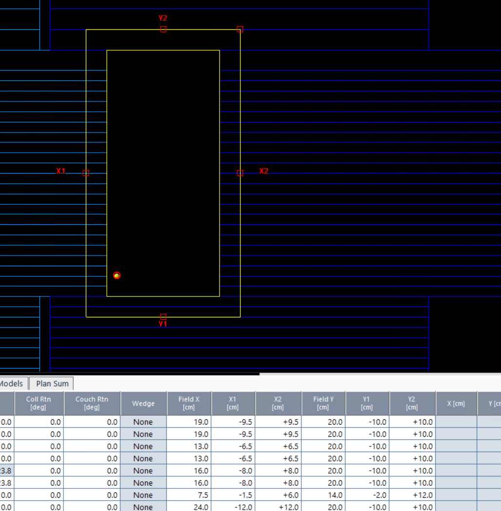
Finally, remember to plot the fluence after generating the plan to ensure it looks as expected. See the Plotting Plan Fluence section for more information.

Open Field¶

Adding an open field can be done like so:

pg.add_open_field_beam(
    x1=-5,
    x2=50,
    y1=-10,
    y2=110,
    defined_by_mlcs=True,
    padding=10,
    beam_name="Open Field",
)

See the add_open_field_beam() method for more information. A jaw-defined field can be created by setting defined_by_mlcs=False. The MLCs will be opened up by the padding value behind the jaws.

Winston-Lutz¶

Winston-Lutz images are open fields, but can be created at given gantry, collimator, and couch angles more efficiently. Adding a Winston-Lutz field can be done like so:

pg.add_winston_lutz_beams(
    axes_positions=(
        {"gantry": 0, "collimator": 0, "couch": 0},
        {"gantry": 90, "collimator": 15, "couch": 0},
        {"gantry": 180, "collimator": 0, "couch": 90},
        {"gantry": 270, "collimator": 0, "couch": 0},
    ),
    x1=-5,
    x2=5,
    y1=-5,
    y2=5,
    defined_by_mlcs=True,
    mu=5,
)

This will create 4 open fields of a 1x1cm, MLC-defined WL fields. See the add_winston_lutz_beams() method for more information.

Picket Fence¶

Adding a picket fence field can be done like so:

pg.add_picketfence_beam(
    strip_width=3,
    strip_positions=(-50, -25, 25, 50),  # 4 pickets
    mu=100,
    beam_name="PF 3mm",
    y1=-130,
    y2=130,  # set y-jaws so we can leave the EPID at 1500
    gantry_angle=90,
    collimator_angle=0,
)

This will create 4 pickets 3mm wide. The X-jaws will be opened up just wider than the pickets. See the add_picketfence_beam() method for more information.

Note

Setting positions too wide can cause an MLC tail exposure, which can cause an issue of deliverability at the Machine. Don’t make the picket positions super far apart. If you want to deliver pickets far away from 0, shift all the pickets over. E.g. (-180, -160, -140, -120).

Dose Rate¶

Adding a single-image dose rate linearity field can be done like so:

pg.add_dose_rate_beams(
    dose_rates=(100, 200, 400, 600),
    y1=-50,
    y2=50,
    mu=100,
    default_dose_rate=600,
    desired_mu=100,
)

This will create 4 ROIs centered about the CAX at different dose rates. A second reference field will also be created. This second field will deliver the same plan but at the default dose rate for all ROIs. This makes the comparison of the ROIs easier than an simple open field.

See the add_dose_rate_beams() method for more information.

MLC Speed¶

Adding an MLC speed field can be done like so:

pg.add_mlc_speed_beams(
    speeds=(5, 10, 15, 20),
    roi_size_mm=20,
    y1=-50,
    y2=50,
    mu=100,
    default_dose_rate=600,
)

This is similar to the dose rate beams, except the modulation occurs to target the MLC speed. A second field is also created where the speed is the maximum speed of the MLCs. See the add_mlc_speed_beams() method for more information.

Note

The typical VMAT plan from Varian that tests gantry-speed/MLC-speed is just that: VMAT. The two variables are intertwined. This test isolates those variables so that just the MLC speed can be tested.

Gantry Speed¶

Adding a gantry speed field can be done like so:

pg.add_gantry_speed_beams(
    speeds=(1, 2, 3, 4),
    max_dose_rate=600,
    start_gantry_angle=179,
    roi_size_mm=20,
    y1=-50,
    y2=50,
    mu=100,
)

This will create multiple ROIs at different gantry speeds. The ROIs themselves are simple, open deliveries. The point here is to only test the gantry speed. The MLCs are not moving during beam-on.

Note

The typical VMAT plan from Varian that tests gantry-speed/dose rate is just that: VMAT. The two variables are intertwined. This test isolates those variables so that just the gantry speed can be tested.

API Documentation¶

class pylinac.plan_generator.dicom.PlanGenerator(ds: Dataset, plan_label: str, plan_name: str, x_width_mm: float = 400, max_mlc_speed: float = 25, max_gantry_speed: float = 4.8, sacrificial_gap_mm: float = 5, max_sacrificial_move_mm: float = 50, max_overtravel_mm: float = 140)[source]¶

Bases: object

A tool for generating new QA RTPlan files based on an initial, somewhat empty RTPlan file.

Parameters¶

dsDataset: The RTPLAN dataset to base the new plan off of. The plan must already have MLC positions.
plan_labelstr: The label of the new plan.
plan_namestr: The name of the new plan.
x_width_mmfloat: The overall width of the MLC movement in the x-direction. Generally, this is the x field size.
max_mlc_speedfloat: The maximum speed of the MLC leaves in mm/s
max_gantry_speedfloat: The maximum speed of the gantry in degrees/s.
sacrificial_gap_mmfloat: For certain dynamic beams, the top and bottom leaf pair are used to slow axes down. This is the gap between those leaves at any given time.
max_sacrificial_move_mmfloat: The maximum distance the sacrificial leaves can move in a given control point. Smaller values generate more control points and more back-and-forth movement. Too large of values may cause deliverability issues.
max_overtravel_mmfloat: The maximum distance the MLC leaves can overtravel from each other as well as the jaw size (for tail exposure protection).

classmethod from_rt_plan_file(rt_plan_file: str, **kwargs) → PlanGenerator[source]¶

Load an existing RTPLAN file and create a new plan based on it.

Parameters¶

rt_plan_filestr: The path to the RTPLAN file.
kwargs: See the PlanGenerator constructor for details.

property num_leaves: int¶: The number of leaves in the MLC.

property leaf_config: list[float]¶: The leaf boundaries of the MLC.

property machine_name: str¶: The name of the machine.

add_beam(beam_dataset: Dataset, mu: int)[source]¶: Add a beam to the plan using the Beam object. Although public, this is a low-level method that is used by the higher-level methods like add_open_field_beam. This handles the associated metadata like the referenced beam sequence and fraction group sequence.

add_picketfence_beam(strip_width_mm: float = 3, strip_positions_mm: tuple[float] = (-45, -30, -15, 0, 15, 30, 45), y1: float = -100, y2: float = 100, fluence_mode: FluenceMode = FluenceMode.STANDARD, dose_rate: int = 600, energy: float = 6, gantry_angle: float = 0, coll_angle: float = 0, couch_vrt: float = 0, couch_lng: float = 1000, couch_lat: float = 0, couch_rot: float = 0, mu: int = 200, jaw_padding_mm: float = 10, beam_name: str = 'PF')[source]¶

Add a picket fence beam to the plan.

Parameters¶

strip_width_mmfloat: The width of the strips in mm.
strip_positions_mmtuple: The positions of the strips in mm relative to the center of the image.
y1float: The bottom jaw position. Usually negative. More negative is lower.
y2float: The top jaw position. Usually positive. More positive is higher.
fluence_modeFluenceMode: The fluence mode of the beam.
dose_rateint: The dose rate of the beam.
energyfloat: The energy of the beam.
gantry_anglefloat: The gantry angle of the beam.
coll_anglefloat: The collimator angle of the beam.
couch_vrtfloat: The couch vertical position.
couch_lngfloat: The couch longitudinal position.
couch_latfloat: The couch lateral position.
couch_rotfloat: The couch rotation.
muint: The monitor units of the beam.
jaw_padding_mmfloat: The padding to add to the X jaws.
beam_namestr: The name of the beam.

add_dose_rate_beams(dose_rates: tuple[int] = (100, 300, 500, 600), default_dose_rate: int = 600, gantry_angle: float = 0, desired_mu: int = 50, energy: float = 6, fluence_mode: FluenceMode = FluenceMode.STANDARD, coll_angle: float = 0, couch_vrt: float = 0, couch_lat: float = 0, couch_lng: float = 1000, couch_rot: float = 0, jaw_padding_mm: float = 5, roi_size_mm: float = 25, y1: float = -100, y2: float = 100)[source]¶

Create a single-image dose rate test. Multiple ROIs are generated. A reference beam is also created where all ROIs are delivered at the default dose rate for comparison. The field names are generated automatically based on the min and max dose rates tested.

Parameters¶

dose_ratestuple: The dose rates to test in MU/min. Each dose rate will have its own ROI.
default_dose_rateint: The default dose rate. Typically, this is the clinical default. The reference beam will be delivered at this dose rate for all ROIs.
gantry_anglefloat: The gantry angle of the beam.
desired_muint: The desired monitor units to deliver. It can be that based on the dose rates asked for, the MU required might be higher than this value.
energyfloat: The energy of the beam.
fluence_modeFluenceMode: The fluence mode of the beam.
coll_anglefloat: The collimator angle of the beam.
couch_vrtfloat: The couch vertical position.
couch_latfloat: The couch lateral position.
couch_lngfloat: The couch longitudinal position.
couch_rotfloat: The couch rotation.
jaw_padding_mmfloat: The padding to add to the X jaws. The X-jaws will close around the ROIs plus this padding.
roi_size_mmfloat: The width of the ROIs in mm.
y1float: The bottom jaw position. Usually negative. More negative is lower.
y2float: The top jaw position. Usually positive. More positive is higher.

add_mlc_speed_beams(speeds: tuple[float] = (5, 10, 15, 20), roi_size_mm: float = 20, mu: int = 50, default_dose_rate: int = 600, gantry_angle: float = 0, energy: float = 6, coll_angle: float = 0, couch_vrt: float = 0, couch_lat: float = 0, couch_lng: float = 1000, couch_rot: float = 0, fluence_mode: FluenceMode = FluenceMode.STANDARD, jaw_padding_mm: float = 5, y1: float = -100, y2: float = 100, beam_name: str = 'MLC Speed')[source]¶

Create a single-image MLC speed test. Multiple speeds are generated. A reference beam is also generated. The reference beam is delivered at the maximum MLC speed.

Parameters¶

speedstuple[float]: The speeds to test in mm/s. Each speed will have its own ROI.
roi_size_mmfloat: The width of the ROIs in mm.
muint: The monitor units to deliver.
default_dose_rateint: The dose rate used for the reference beam.
gantry_anglefloat: The gantry angle of the beam.
energyint: The energy of the beam.
coll_anglefloat: The collimator angle of the beam.
couch_vrtfloat: The couch vertical position.
couch_latfloat: The couch lateral position.
couch_lngfloat: The couch longitudinal position.
couch_rotfloat: The couch rotation.
fluence_modeFluenceMode: The fluence mode of the beam.
jaw_padding_mmfloat: The padding to add to the X jaws. The X-jaws will close around the ROIs plus this padding.
y1float: The bottom jaw position. Usually negative. More negative is lower.
y2float: The top jaw position. Usually positive. More positive is higher.
beam_namestr: The name of the beam. The reference beam will be called “MLC Sp Ref”.

Notes¶

The desired speed can be achieved through the following formula:

speed = roi_size_mm * max dose rate / MU * 60

We solve for MU with the desired speed. The 60 is for converting the dose rate as MU/min to MU/sec. Thus,

MU = roi_size_mm * max dose rate / speed * 60

MUs are calculated automatically based on the speed and the ROI size.

add_winston_lutz_beams(x1: float = -10, x2: float = 10, y1: float = -10, y2: float = 10, defined_by_mlcs: bool = True, energy: float = 6, fluence_mode: FluenceMode = FluenceMode.STANDARD, dose_rate: int = 600, axes_positions: Iterable[dict] = ({'collimator': 0, 'couch': 0, 'gantry': 0},), couch_vrt: float = 0, couch_lng: float = 1000, couch_lat: float = 0, mu: int = 10, padding_mm: float = 5)[source]¶

Add Winston-Lutz beams to the plan. Will create a beam for each set of axes positions. Field names are generated automatically based on the axes positions.

Parameters¶

x1float: The left jaw position.
x2float: The right jaw position.
y1float: The bottom jaw position.
y2float: The top jaw position.
defined_by_mlcsbool: Whether the field edges are defined by the MLCs or the jaws.
energyfloat: The energy of the beam.
fluence_modeFluenceMode: The fluence mode of the beam.
dose_rateint: The dose rate of the beam.
axes_positionsIterable[dict]: The positions of the axes. Each dict should have keys ‘gantry’, ‘collimator’, and ‘couch’.
couch_vrtfloat: The couch vertical position.
couch_lngfloat: The couch longitudinal position.
couch_latfloat: The couch lateral position.
muint: The monitor units of the beam.
padding_mmfloat: The padding to add. If defined by the MLCs, this is the padding of the jaws. If defined by the jaws, this is the padding of the MLCs.

add_gantry_speed_beams(speeds: tuple = (2, 3, 4, 4.8), max_dose_rate: int = 600, start_gantry_angle: float = 179, energy: float = 6, fluence_mode: FluenceMode = FluenceMode.STANDARD, coll_angle: float = 0, couch_vrt: float = 0, couch_lat: float = 0, couch_lng: float = 1000, couch_rot: float = 0, beam_name: str = 'GS', gantry_rot_dir: GantryDirection = GantryDirection.CLOCKWISE, jaw_padding_mm: float = 5, roi_size_mm: float = 30, y1: float = -100, y2: float = 100, mu: int = 120)[source]¶

Create a single-image gantry speed test. Multiple speeds are generated. A reference beam is also generated. The reference beam is delivered without gantry movement.

Parameters¶

speedstuple: The gantry speeds to test. Each speed will have its own ROI.
max_dose_rateint: The max dose rate clinically allowed for the energy.
start_gantry_anglefloat: The starting gantry angle. The gantry will rotate around this point. It is up to the user to know what the machine’s limitations are. (i.e. don’t go through 180 for Varian machines). The ending gantry angle will be the starting angle + the sum of the gantry deltas generated by the speed ROIs. Slower speeds require more gantry angle to reach the same MU.
energyfloat: The energy of the beam.
fluence_modeFluenceMode: The fluence mode of the beam.
coll_anglefloat: The collimator angle of the beam.
couch_vrtfloat: The couch vertical position.
couch_latfloat: The couch lateral position.
couch_lngfloat: The couch longitudinal position.
couch_rotfloat: The couch rotation.
beam_namestr: The name of the beam.
gantry_rot_dirGantryDirection: The direction of gantry rotation.
jaw_padding_mmfloat: The padding to add to the X jaws. The X-jaws will close around the ROIs plus this padding.
roi_size_mmfloat: The width of the ROIs in mm.
y1float: The bottom jaw position. Usually negative. More negative is lower.
y2float: The top jaw position. Usually positive. More positive is higher.
muint: The monitor units of the beam.

Notes¶

The gantry angle to cover can be determined via the following:

gantry speed = gantry_range * max_dose_rate / (MU * 60)

We can thus solve for the gantry range:

gantry_range = gantry_speed * MU * 60 / max_dose_rate

add_open_field_beam(x1: float, x2: float, y1: float, y2: float, defined_by_mlcs: bool = True, energy: float = 6, fluence_mode: FluenceMode = FluenceMode.STANDARD, dose_rate: int = 600, gantry_angle: float = 0, coll_angle: float = 0, couch_vrt: float = 0, couch_lng: float = 1000, couch_lat: float = 0, couch_rot: float = 0, mu: int = 200, padding_mm: float = 5, beam_name: str = 'Open', outside_strip_width_mm: float = 5)[source]¶

Add an open field beam to the plan.

Parameters¶

x1float: The left jaw position.
x2float: The right jaw position.
y1float: The bottom jaw position.
y2float: The top jaw position.
defined_by_mlcsbool: Whether the field edges are defined by the MLCs or the jaws.
energyfloat: The energy of the beam.
fluence_modeFluenceMode: The fluence mode of the beam.
dose_rateint: The dose rate of the beam.
gantry_anglefloat: The gantry angle of the beam.
coll_anglefloat: The collimator angle of the beam.
couch_vrtfloat: The couch vertical position.
couch_lngfloat: The couch longitudinal position.
couch_latfloat: The couch lateral position.
couch_rotfloat: The couch rotation.
muint: The monitor units of the beam.
padding_mmfloat: The padding to add to the jaws or MLCs.
beam_namestr: The name of the beam.
outside_strip_width_mmfloat: The width of the strip of MLCs outside the field. The MLCs will be placed to the left, under the X1 jaw by ~2cm.

to_file(filename: str | Path) → None[source]¶: Write the DICOM dataset to file

as_dicom() → Dataset[source]¶: Return the new DICOM dataset.

plot_fluences(width_mm: float = 400, resolution_mm: float = 0.5, dtype: ~numpy.dtype = <class 'numpy.uint16'>) → list[Figure][source]¶: Plot the fluences of the beams generated

See Also¶

plot_fluences()

class pylinac.plan_generator.dicom.Beam(plan_dataset: Dataset, beam_name: str, beam_type: BeamType, energy: float, dose_rate: int, x1: float, x2: float, y1: float, y2: float, machine_name: str, gantry_angles: float | list[float], gantry_direction: GantryDirection, coll_angle: float, couch_vrt: float, couch_lat: float, couch_lng: float, couch_rot: float, mlc_boundaries: list[float], mlc_positions: list[list[float]], metersets: list[float], fluence_mode: FluenceMode)[source]¶

Bases: object

Represents a DICOM beam dataset. Has methods for creating the dataset and adding control points. Generally not created on its own but rather under the hood as part of a PlanGenerator object.

It contains enough independent logic steps that it’s worth separating out from the PlanGenerator class.

Parameters¶

plan_dataset: The plan dataset. Used for dynamic links to other Sequences of the plan, such as Dose Reference and Tolerance Table.
beam_namestr: The name of the beam. Must be less than 16 characters.
beam_typeBeamType: The type of beam: dynamic or static.
energyfloat: The energy of the beam.
dose_rateint: The dose rate of the beam.
x1float: The left jaw position.
x2float: The right jaw position.
y1float: The bottom jaw position.
y2float: The top jaw position.
machine_namestr: The name of the machine.
gantry_anglesUnion[float, list[float]]: The gantry angle(s) of the beam. If a single number, it’s assumed to be a static beam. If multiple numbers, it’s assumed to be a dynamic beam.
gantry_directionGantryDirection: The direction of the gantry rotation. Only relevant if multiple gantry angles are specified.
coll_anglefloat: The collimator angle.
couch_vrtfloat: The couch vertical position.
couch_latfloat: The couch lateral position.
couch_lngfloat: The couch longitudinal position.
couch_rotfloat: The couch rotation.
mlc_boundarieslist[float]: The MLC boundaries. These are the same thing as the LeafPositionBoundaries in the DICOM file.
mlc_positionslist[list[float]]: The MLC positions for each control point. This is the x-position of each leaf for each control point.
metersetslist[float]: The meter sets for each control point. The length must match the number of control points in mlc_positions.
fluence_modeFluenceMode: The fluence mode of the beam.

as_dicom() → Dataset[source]¶: Return the beam as a DICOM dataset that represents a BeamSequence item.

class pylinac.plan_generator.mlc.MLCShaper(leaf_y_positions: list[float], max_x_mm: float, sacrifice_gap_mm: float = 5, sacrifice_max_move_mm: float = 50, max_overtravel_mm: float = 140)[source]¶

Bases: object

The MLC Shaper is a tool for generating MLC positions and sequences to create a given pattern. Meterset values can be given and set. It can also create ‘sacrifices’ of MLC leaves to set the MLC speed/dose rate to a certain value.

Parameters¶

leaf_y_positions: The y-positions of the MLC leaves. This is the same as the LeafJawPositions in the DICOM RT Plan.
max_x_mm: The maximum x-position of the MLC leaves. E.g. 200mm away from the isocenter is 200.
sacrifice_gap_mm: The gap between the sacrificial leaves. This is used to separate the leaves that are being moved out of the way.
sacrifice_max_move_mm: The maximum distance a sacrificial leaf can move in one control point.
max_overtravel_mm: The maximum distance a leaf can move beyond another MLC leaf and also the limit of exposure of the MLC tail.

property centers: list[float]¶: The center positions of the MLC leaves

property num_leaves: int¶: The number of leaves in the MLC

property num_pairs: int¶: The number of leaf pairs in the MLC

as_control_points() → list[list[float]][source]¶: Return the MLC positions in DICOM format as a list of positions for each control point

as_metersets() → list[float][source]¶: Return the MLC metersets in DICOM format as a list for each control point

add_rectangle(left_position: float, right_position: float, x_outfield_position: float, top_position: float, bottom_position: float, outer_strip_width: float, meterset_at_target: float, meterset_transition: float = 0, sacrificial_distance: float = 0, initial_sacrificial_gap: float | None = None) → None[source]¶

Create a rectangle using the MLCs.

Parameters¶

left_position: The left positions the MLCs should have when they are on the “infield” area in mm
right_position: The right side of the rectangle in mm.
x_outfield_position: The position the MLCs should have when they are on the “outfield” area. Typically, these are unused/outside leaves and just need to be put somewhere.
top_position: The upper y-bound that defines the out/in boundary in mm.
bottom_position: The lower y-bound that defines the out/in boundary in mm.
outer_strip_width: The separation width in mm of the leaves for the leaves outside the rectangle.
meterset_at_target: The ratio of MU that should be delivered AT the target rectangle position. This is for delivered rectangles of dose. E.g. for a picket fence the meterset at target might be 0.25 to deliver 25% of the dose at each picket.
meterset_transition: The ratio of MU that should be delivered between the MLC state before the rectangle and the MLC state AT the target rectangle position. Set to 0 to transition immediately without dose. E.g. if delivering a picket fence the dose between pickets is low or 0. For an MLC speed test or an ROI where the goal is to deliver through a transition region, this might be high compared to the meterset at target.
sacrificial_distance: The distance to move the sacrificial leaves. This is used to module the dose rate or MLC speed. If this is set, the meterset_transition must be set to a non-zero value.
initial_sacrificial_gap: The initial gap between the sacrificial leaves. This is only used for the first control point.

add_strip(position_mm: float, strip_width_mm: float, meterset_at_target: float, meterset_transition: float = 0, sacrificial_distance_mm: float = 0, initial_sacrificial_gap_mm: float | None = None) → None[source]¶

Create a single strip composed of MLCs. This is a subset of the add_rectangle method, but centers the strip about the x_infield_position and uses all the leaves.

Parameters¶

position_mm: The central x-position of the leaves for the leaves on the ‘infield’ in mm.
strip_width_mm: The width of the strip in mm, centered about the x_infield_position.
meterset_at_target: The ratio of MU that should be delivered within this control point. Set to 0 for a “transition” control point, such as at the beginning or end of a beam or when moving from one ROI to another.
meterset_transition: The ratio of MU that should be delivered between the MLC state before the strip and the MLC state AT the target strip position. Set to 0 to transition immediately without dose. E.g. if delivering a picket fence the dose between pickets is low or 0. For an MLC speed test or an ROI where the goal is to deliver through a transition region, this might be high compared to the meterset at target.
sacrificial_distance_mm: The distance to move the sacrificial leaves. This is used to module the dose rate. If this is set, the meterset_transition must be set to a non-zero value.
initial_sacrificial_gap_mm: The initial gap between the sacrificial leaves. This is only used for the first control point.

Plan Generator¶

Prerequisites¶

Typical Use¶

Plotting Fluence¶

Delivering the Plan¶

Models¶

Overview¶

Plan Generator¶

MLC Shaper¶

Beam¶

Sacrifices¶

Fields¶

Open Field¶

Winston-Lutz¶

Picket Fence¶

Dose Rate¶

MLC Speed¶

Gantry Speed¶

API Documentation¶

Parameters¶

Parameters¶

Parameters¶

Parameters¶

Parameters¶

Notes¶

Parameters¶

Parameters¶

Notes¶

Parameters¶

See Also¶

Parameters¶

Parameters¶

Parameters¶

Parameters¶