Images & 2D Metrics
Added in version 3.16.
Pylinac images can now have arbitrary metrics calculated on them, similar to profiles. This can be useful for calculating and finding values and regions of interest in images. The system is quite flexible and allows for any number of metrics to be calculated on an image. Furthermore, this allows for re-usability of metrics, as they can be applied to any image.
Use Cases
Calculate the mean pixel value of an area of an image.
Finding an object in the image.
Calculating the distance between two objects in an image.
Tool Legend
Tools can be divided into two categories: Finders and Samplers. The main difference is that Finders are used to locate objects in the image (using image features/pixel data) and Samplers are used to sample the image in some way where the location of the ROI is known or fixed. Finders make use of image features while Samplers do not.
Finders use image features to locate objects in the image, such as a BB or field. From here, a user may then want to calculate properties of the object, such as the area or weighted centroid.
Samplers are tools that sample the image in some way, such as calculating the mean pixel value of a region. These are not mutually exclusive use cases. E.g. a Finder may be used to locate a BB and then a Sampler may be used to calculate the mean pixel value of the region around that ROI or sample an offset from it, such as the penumbra or background.
Finders
Use Case |
Constraint |
Class |
|---|---|---|
Find the location of a single BB in the image |
The BB size and location is known approximately |
|
Find the locations of N BBs in the image |
The BB sizes are all similar and location is known approximately |
|
Find the ROI properties of a single BB in the image |
The BB size and location is known approximately |
|
Find the ROI properties of N BBs in the image |
The BB size and location is known approximately |
|
Find the location of a single BB anywhere in the image |
The BB size is known approximately |
|
Find the locations of N BBs anywhere in the image |
The BB size is known approximately |
|
Find the location of a square field in an image |
The field size is known approximately |
|
Find the locations of N square fields in an image |
The field size is known approximately |
|
Find the locations of N square fields in an image |
The field size is not known |
|
Find the location of a circular field in an image |
The field size and location are known approximately |
|
Find the ROI properties of a circular field in an image |
The field size and location are known approximately |
|
Samplers
DiskROIMetric: Sample a circular region of interest. Will return aDiskROIobject. This object contains the mean pixel value, standard deviation, and other properties of the ROI.RectangleROIMetric: Sample a rectangular region of interest. Will return aRectangleROIobject. This object contains the mean pixel value, standard deviation, and other properties of the ROI.
Basic Usage
To calculate metrics on an image, simply pass the metric(s) to the compute method of the image:
from pylinac.core.image import DicomImage
from pylinac.metrics.image import DiskLocator, DiskRegion

img = DicomImage("my_image.dcm")
metric = img.compute(
    metrics=DiskLocator(
        expected_position=(100, 100),
        search_window=(30, 30),
        radius=10,
        radius_tolerance=2,
    )
)
print(metric)
You may compute multiple metrics by passing a list of metrics:
from pylinac.core.image import DicomImage
from pylinac.metrics.image import DiskLocator, DiskRegion

img = DicomImage("my_image.dcm")
metrics = img.compute(
    metrics=[
        # disk 1
        DiskLocator(
            expected_position=(100, 100),
            search_window=(30, 30),
            radius=10,
            radius_tolerance=2,
        ),
        # disk 2
        DiskLocator(
            expected_position=(200, 200),
            search_window=(30, 30),
            radius=10,
            radius_tolerance=2,
        ),
    ]
)
print(metrics)
Metrics might have something to plot on the image. If so, the plot method of the image will plot the metric(s) on the image:
from pylinac.core.image import DicomImage
from pylinac.metrics.image import DiskLocator, DiskRegion

img = DicomImage("my_image.dcm")
metrics = img.compute(
    metrics=[
        # disk 1
        DiskLocator(
            expected_position=(100, 100),
            search_window=(30, 30),
            radius=10,
            radius_tolerance=2,
        ),
        # disk 2
        DiskLocator(
            expected_position=(200, 200),
            search_window=(30, 30),
            radius=10,
            radius_tolerance=2,
        ),
    ]
)
img.plot()  # plots the image with the BB positions overlaid
Built-in Metrics
Sized Disk Locator
Note
The values provided below are in pixels. The following sections show how variants of how to use the metrics using physical units and relative to the center of the image.
Here’s an example of using the SizedDiskLocator:
from pylinac.core.image import DicomImage
from pylinac.metrics.image import DiskLocator, DiskRegion

img = DicomImage("my_image.dcm")
img.compute(
    metrics=[
        DiskLocator(
            expected_position=(100, 100),
            search_window=(30, 30),
            radius=10,
            radius_tolerance=2,
        )
    ]
)
img.plot()
This will search for a disk (BB) in the image at the expected position and window size for a disk of a given radius and tolerance.
If the disk is found, the location will be returned as a Point object.
If the disk is not found, a ValueError will be raised.
Using physical units
While pixels are useful, it is sometimes easier to use physical units.
To perform the same Disk/BB location using mm instead of pixels:
from pylinac.core.image import DicomImage
from pylinac.metrics.image import DiskLocator, DiskRegion

img = DicomImage("my_image.dcm")
img.compute(
    metrics=[
        # these are all in mm
        DiskLocator.from_physical(
            expected_position_mm=(30, 30),
            search_window_mm=(10, 10),
            radius_mm=4,
            radius_tolerance_mm=2,
        )
    ]
)
img.plot()
Relative to center
We can also specify the expected position relative to the center of the image.
Important
We can do this using pixels OR physical units.
This will look for the disk/BB 30 pixels right and 30 pixels down from the center of the image:
from pylinac.core.image import DicomImage
from pylinac.metrics.image import DiskLocator, DiskRegion

img = DicomImage("my_image.dcm")
img.compute(
    metrics=[
        # these are all in pixels
        DiskLocator.from_center(
            expected_position=(30, 30),
            search_window=(10, 10),
            radius=4,
            radius_tolerance=2,
        )
    ]
)
img.plot()
This will look for the disk/BB 30mm right and 30mm down from the center of the image:
img.compute(
    metrics=[
        # these are all in mm
        DiskLocator.from_center_physical(
            expected_position_mm=(30, 30),
            search_window_mm=(10, 10),
            radius_mm=4,
            radius_tolerance_mm=2,
        )
    ]
)
img.plot()
Sized Disk Region
The SizedDiskRegion metric is the same as the SizedDiskLocator, but instead of returning the location, it returns a
scikit-image regionprops object that is the region of the disk.
This allows one to then calculate things like the weighted centroid, area, etc.
It also supports the same class methods as the SizedDiskLocator metric.
Global Sized Disk Locator
Added in version 3.17.
The GlobalSizedDiskLocator metric is similar to the SizedDiskLocator metric
except that it searches the entire image for disks/BB, not just a small window. This is useful for finding the BB in images
where the BB is not in the expected location or unknown. This is also efficient for finding BBs in images,
even if the locations are known.
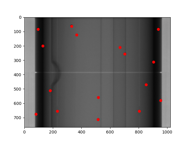
For example, here is an example analysis of an MPC image:
from pylinac.core.image import XIM
from pylinac.metrics.image import GlobalDiskLocator

img = XIM("my_image.xim")
bbs = img.compute(
    metrics=GlobalDiskLocator(
        radius_mm=3.5,
        radius_tolerance_mm=1.5,
        min_number=10,
    )
)
img.plot()
This will result in an image like so:
Global Sized Field Locator
Added in version 3.17.
The GlobalSizedFieldLocator metric is similar to the GlobalSizedDiskLocator metric.
This is useful for finding one or more fields in images
where the field is not in the expected location or unknown. This is also efficient when multiple fields are present in the image.
The locator will find the weighted center of the field(s) and return the location(s) as a Point objects.
The boundary of the detected field(s) will be plotted on the image in addition to the center.
The locator will use pixels by default, but also has a from_physical class method to use physical units.
An example plot of finding multiple fields can be seen below:
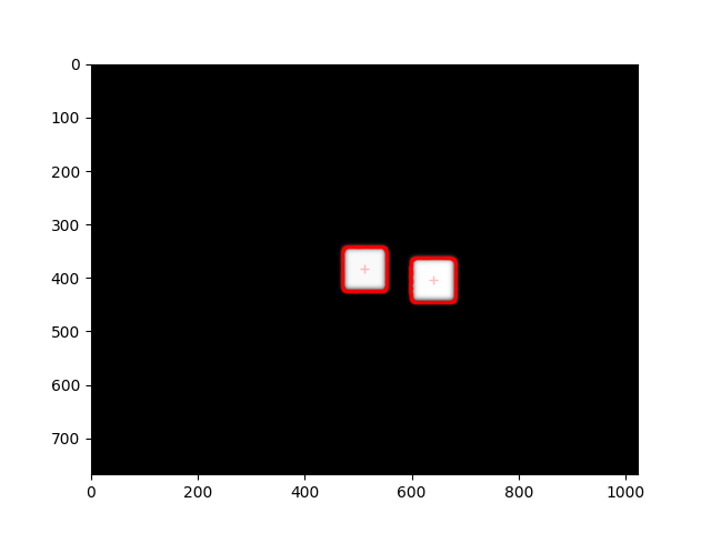
For example:
img = DicomImage("my_image.dcm")
img.compute(
    metrics=GlobalSizedFieldLocator(
        field_width_px=30, field_height_px=30, field_tolerance_px=4, max_number=2
    )
)
img.plot()  # this will plot the image with the fields overlaid
Constraints
The field is expected to be mostly rectangular. I.e. not a cone.
The field must not be touching an edge of the image. Such fields will be ignored.
The field must be at least 10% of the maximum pixel value. This is to avoid finding artifacts. I.e. If the maximum pixel value is 10,000, then the pixels within the field must be at least 1,000 to be detected. Anything under 10% will be ignored.
Using physical units
To perform a similar field location using mm instead of pixels:
img = DicomImage("my_image.dcm")
img.compute(
    metrics=GlobalSizedFieldLocator.from_physical(
        field_width_mm=30, field_height_mm=30, field_tolerance_mm=4, max_number=2
    )
)
Usage tips
Whenever possible, set the
max_numberparameter. This can greatly speed up the computation for several reasons. First, it will stop searching once the number of fields is found. Second, the thresholding algorithm will have a much better initial guess and also a better step size. This is because the approximate area of the field is known relative to the total image size.The
field_tolerance_<mm|px>parameter can be relatively tight if themax_numberparameter is set. Without amax_numberparameter, you may have to increase the field tolerance to find all fields.
Global Field Locator
Added in version 3.17.
The GlobalFieldLocator metric will find fields within an image, but does not require the field to be a specific size.
It will find anything field-like in the image. The logic is similar to the GlobalSizedFieldLocator metric otherwise.
The position can be specified in pixels or mm.
For example:
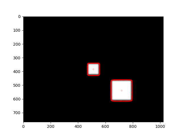
img = DicomImage("my_image.dcm")
img.compute(metrics=GlobalFieldLocator(max_number=2))
img.plot()  # this will plot the image with the fields overlaid
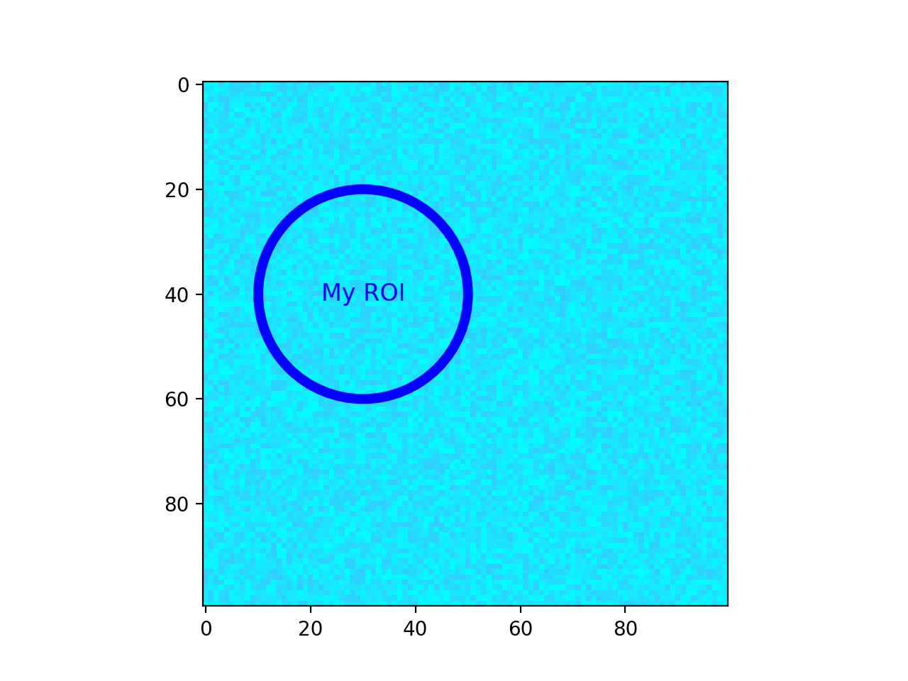
Disk ROI Metric
Added in version 3.25.
The DiskROIMetric metric will sample a circular region of interest (ROI) in the image.
This will return a DiskROI object. This object can then be used to
determine the mean pixel value, standard deviation, etc.
As with the other metrics, this can be specified in pixels or mm.
import numpy as np

from pylinac.core.roi import DiskROI
from pylinac.core.image import DicomImage
from pylinac.metrics.image import DiskROIMetric

img = DicomImage("my_image.dcm")

# position in pixels
roi: DiskROI = img.compute(
    metrics=DiskROIMetric(
        radius=20,
        center=Point(511.5, 383.5),
    )
)
img.plot()

mean = np.mean(roi.pixel_values)

# position in mm
roi: DiskROI = img.compute(
    metrics=DiskROIMetric.from_physical(
        radius_mm=10,
        center_mm=(70, 80),
    )
)
(Source code, png, hires.png, pdf)
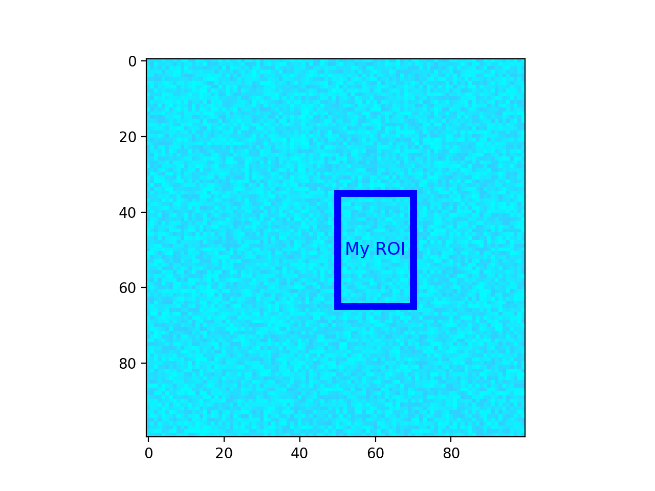
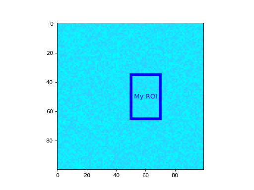
Rectangle ROI Metric
Added in version 3.25.
The RectangleROIMetric metric will sample a rectangular region of interest (ROI) in the image.
This will return a RectangleROI object. This object can then be used to
determine the mean pixel value, standard deviation, etc.
As with the other metrics, this can be specified in pixels or mm.
import numpy as np

from pylinac.core.roi import RectangleROI
from pylinac.core.image import DicomImage
from pylinac.metrics.image import RectangleROIMetric

img = DicomImage("my_image.dcm")

# position in pixels
roi: RectangleROI = img.compute(
    metrics=RectangleROIMetric(
        width=20,
        height=30,
        center=Point(511.5, 383.5),
    )
)
img.plot()

mean = np.mean(roi.pixel_array)

# position in mm
roi: RectangleROI = img.compute(
    metrics=RectangleROIMetric.from_physical(
        width_mm=10,
        height_mm=20,
        center_mm=(70, 80),
    )
)
(Source code, png, hires.png, pdf)
Writing Custom Plugins
The power of the plugin architecture is that you can write your own metrics and use them on any image as well as reuse them where needed.
To write a custom plugin, you must
Inherit from the
MetricBaseclassSpecify a
nameattribute.Implement the
calculatemethod.(Optional) Implement the
plotmethod if you want the metric to plot on the image.
Warning
Do not modify the image in the calculate method as this will affect the image for other metrics and/or plotting.
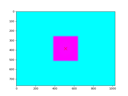
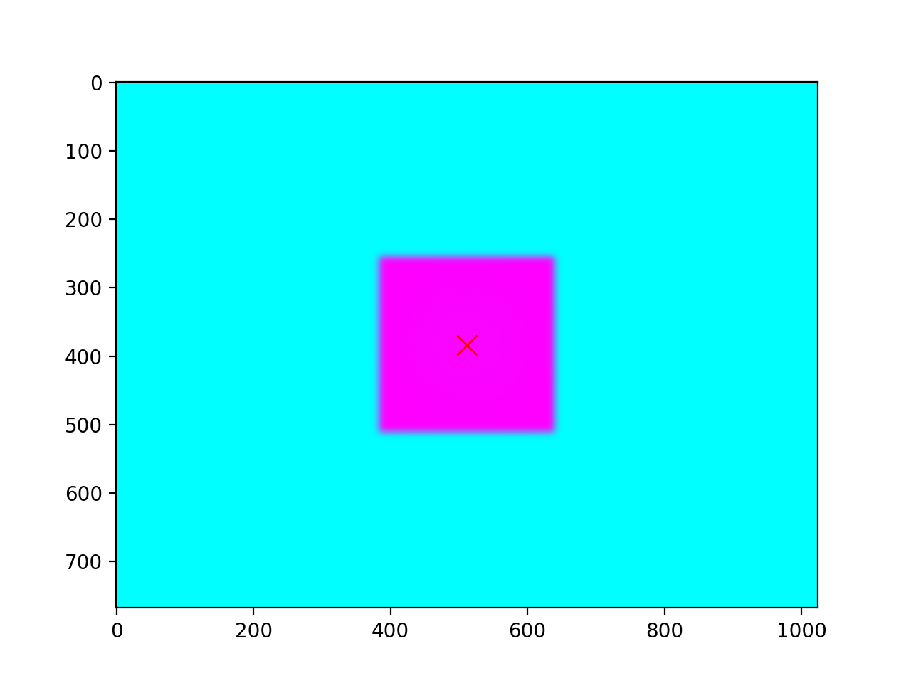
For example, let’s built a simple plugin that finds and plots an “X” at the center of the image:
from pylinac.core.image_generator import AS1000Image, FilteredFieldLayer, GaussianFilterLayer
from pylinac.core.image import DicomImage
from pylinac.metrics.image import MetricBase

class ImageCenterMetric(MetricBase):
    name = "Image Center"

    def calculate(self):
        return self.image.center

    def plot(self, axis: plt.Axes):
        axis.plot(self.image.center.x, self.image.center.y, 'rx', markersize=10)

# now we create an image to compute over
as1000 = AS1000Image(sid=1000)  # this will set the pixel size and shape automatically
as1000.add_layer(
    FilteredFieldLayer(field_size_mm=(100, 100))
)  # create a 100x100mm square field
as1000.add_layer(
    GaussianFilterLayer(sigma_mm=2)
)  # add an image-wide gaussian to simulate penumbra/scatter
ds = as1000.as_dicom()

# now we can compute the metric on the image
img = DicomImage.from_dataset(ds)
center = img.compute(metrics=ImageCenterMetric())
print(center)
img.plot()
(Source code, png, hires.png, pdf)

Algorithm
The algorithms for the metrics are similar to each other. They all use a thresholding algorithm to find the object(s) of interest. For the example below, we will be using the first image from the Winston Lutz demo dataset:
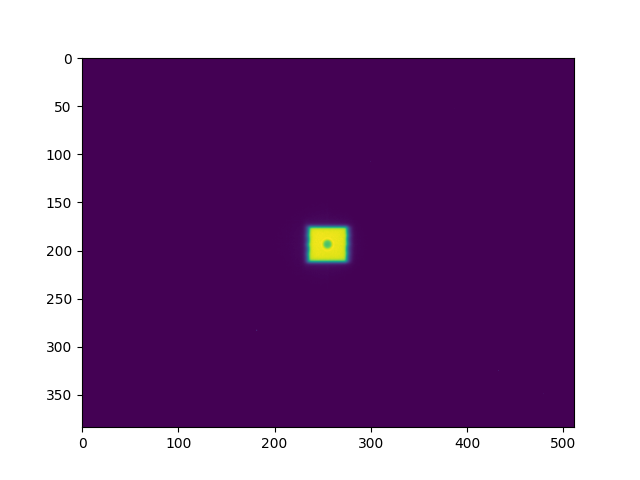
Original image to be analyzed.
The image is cropped if needed. This applies to metrics that have an expected position. I.e. non-
Globalvariants of the metrics. This cropped section is called the “sample”.Important
Image analyses using the
WinstonLutzclass are always cropped like this.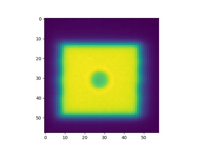
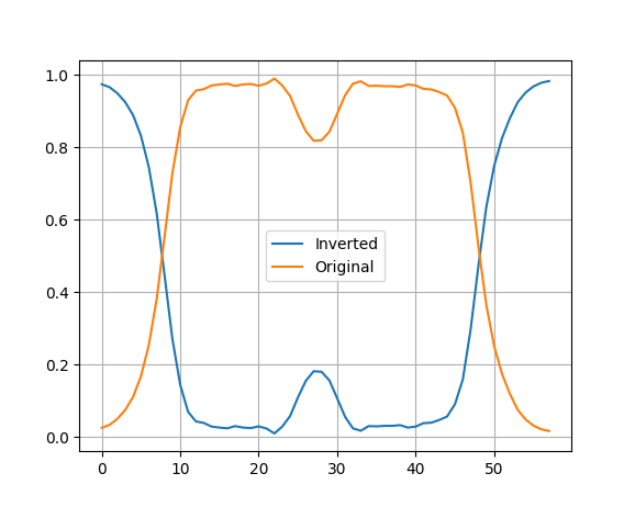
The sample might be inverted depending on the
invertparameter. This applies to disk/BB metrics. The reason for inversion is that in the case of a BB within an open field, the pixel values within the BB ROI will be lower than the field surrounding it. Because pylinac uses weighted pixel values to find the center of the object, the pixel values need to be proportional to the “impact” of the object.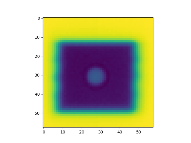
To make this clear, the profiles are plotted below with and without inversion. Because pylinac uses the weighted centroid of the pixels, we want the BB to “weigh” more at the center than the edges of the BB.
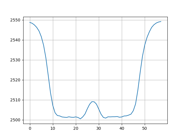
The sample is normalized to a range of 0-1. This is done because sometimes the attenuation of a BB can be relatively small compared to the surrounding field. Doing so ensures the central pixels’ weighting is large and the BB edge pixel values is relatively small.
Note
For
Globalmetrics, this often won’t change the image very much since the entire image is searched.The image below shows why normalization is helpful. When not normalized, the BB pixel values can be very similar to the region outside the BB. E.g. the value at index 20 (outside the BB in the field area) is ~2502 while the peak BB value at index 27 is ~2509. With such a small difference, the weighted centroid will be very similar to a simple centroid, which is not as accurate as it’s sensitive to “edge” pixels of the blob.
The image is then converted to binary using a threshold. The threshold starts at 0.02. E.g. for this threshold value any pixel below 0.02 is set to 0 and everything above it is set to 1. The resulting binary image is analyzed to see if each “blob” passed all of the
detection_conditions.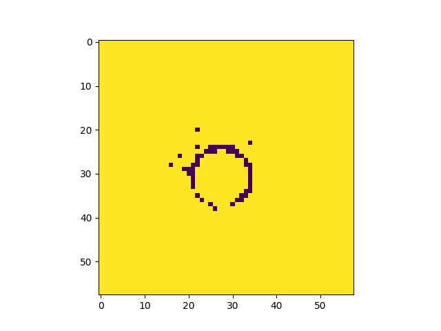
The detection conditions can be anything and generally measure blob properties such as area, eccentricity, etc. Each blob is a regionprops . The blob has a vast number of properties that are calculated and can be measured. E.g. the disk detection conditions are that the blob is 1) round, 2) has an area within the expected range given the BB size, and 3) has a circumference within the expected range given the BB size.
The image above isn’t very helpful because the BB isn’t really visible here.
If no blob passes all the detection conditions, the threshold is increased by 0.02 and the process is repeated.
Here is the image when the detection conditions pass:
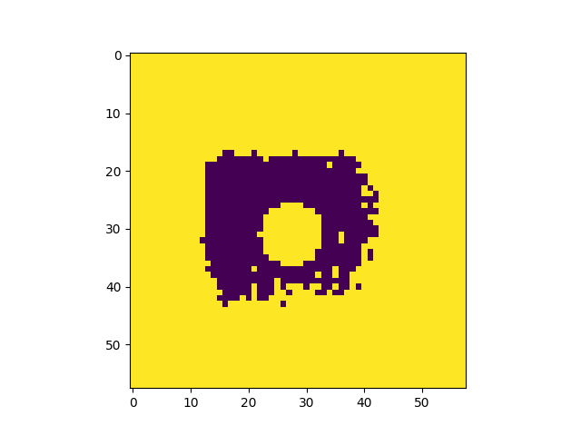
Clearly, this threshold works well and the BB is identifiable.
If there is a
max_numberparameter, the thresholding algorithm will stop once that number is reached. This is because the thresholding algorithm can be slow, and once the expected number of objects is found there is no need to continue.Important
Setting a
max_numberdoes not guarantee that only that number of objects will be found. It only guarantees that once that number is found, the thresholding algorithm will stop. This is because the thresholding algorithm could find multiple objects at a given threshold value.If the
max_numberparameter is not set, the thresholding algorithm will continue until the threshold reaches 1.0.If the
min_numberparameter is set and the thresholding algorithm stops (i.e. reaches 1.0), aValueErroris raised.Note
The
min_numberandmax_numberparameters are only available for theGlobalvariants of the metrics. They are both fixed to 1 for single object metrics.If no blobs are found that match all the detection conditions after the threshold reaches 1.0, a
ValueErroris raised.For each blob that is detected, the boundary of the binary threshold of that blob is tracked. This is solely used for plotting.
At each pass of the threshold, if more objects are detected, they are compared and potentially de-duplicated. This is because if, e.g., we are looking for two objects and one is found at a given threshold, it will likely continue to be found again and again at higher thresholds while we are searching for the second object.
This comparison is done by comparing the centroids of the blobs. If the centroids are within the
min_separation_mm, the first blob is retained and the subsequent blob is discarded. If the centroid is sufficiently far away, the blob is retained.Note that it’s also possible the original blob is no longer seen at higher thresholds. E.g. multiple small fields each delivering different MUs. In all cases, regions/points are always kept even if it is no longer detected at higher thresholds. I.e. the regions/points are add-only.
For
Locatormetrics, the weighted centroid of the blob is returned as aPointobject. ForRegionmetrics, the scikit-image regionprops object is returned.Important
I can’t stress this enough: the weighted centroid is not the same as the simple centroid. The weighted centroid is the centroid of the blob accounting for the pixel value itself. This will not be nearly as sensitive to “edge” pixels being included as a simple centroid. The simple centroid is the average of the pixel locations not accounting for the pixel value. You will find some other commercial software uses only the simple centroid, which is not as accurate as it’s far more sensitive to edge pixels being included in the threshold.
Here is the plot of the final image with the BB location and threshold boundary overlaid:
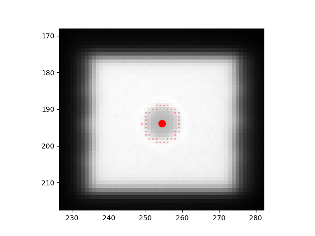
Note
Note the single pixel on the left side boundary of the BB. A different threshold may or may not have included that pixel. The benefit of the weighted centroid is that the normalized, inverted sample value at that pixel is ~0 whereas the pixels at the center of the BB are ~1. The weighted centroid thus is hardly affected by that pixel, so it’s robust to a change in threshold.
API
Finders
- class pylinac.metrics.image.MetricBase[source]
Bases:
ABCBase class for any 2D metric. This class is abstract and should not be instantiated.
The subclass should implement the
calculatemethod and thenameattribute.As a best practice, the
image_compatibilityattribute should be set to a list of image classes that the metric is compatible with. Image types that are not in the list will raise an error. This allows compatibility to be explicit. However, by default this is None and no compatibility checking is done.
- class pylinac.metrics.image.SizedDiskLocator(expected_position: ~pylinac.core.geometry.Point | tuple[float, float], search_window: tuple[float, float], radius: float, radius_tolerance: float, detection_conditions: list[~collections.abc.Callable[[~skimage.measure._regionprops.RegionProperties, ...], bool]] = (<function is_right_size_bb>, <function is_round>, <function is_right_circumference>, <function is_symmetric>, <function is_solid>), invert: bool = True, name: str = 'Disk Region', max_number: int = 1, min_number: int = 1, min_separation_pixels: float = 5)[source]
Bases:
SizedDiskRegionCalculates the weighted centroid of a disk/BB as a Point in an image where the disk is near an expected position and size.
- plotly(fig: Figure, show_boundaries: bool = True, color: str = 'red', marker_size: float = 7, opacity: float = 0.25, **kwargs) None[source]
Plot the BB center
- plot(axis: Axes, show_boundaries: bool = True, color: str = 'red', markersize: float = 3, alpha: float = 0.25) None[source]
Plot the BB center
- additional_plots() list[figure]
Plot additional information on a separate figure as needed.
This should NOT show the figure. The figure will be shown via the
metric_plotsmethod. Calling show here would block other metrics from plotting their own separate metrics.
- context_calculate() Any
Calculate the metric. This also checks the image hash to attempt to ensure no changes were made.
- classmethod from_center(expected_position: ~pylinac.core.geometry.Point | tuple[float, float], search_window: tuple[float, float], radius: float, radius_tolerance: float, detection_conditions: list[~collections.abc.Callable[[~skimage.measure._regionprops.RegionProperties, ...], bool]] = (<function is_right_size_bb>, <function is_round>, <function is_right_circumference>, <function is_symmetric>, <function is_solid>), invert: bool = True, name='Disk Region', max_number: int = 1, min_number: int = 1, min_separation_pixels: float = 5)
Create a DiskRegion from a center point.
- classmethod from_center_physical(expected_position_mm: ~pylinac.core.geometry.Point | tuple[float, float], search_window_mm: tuple[float, float], radius_mm: float, radius_tolerance_mm: float = 0.25, detection_conditions: list[~collections.abc.Callable[[~skimage.measure._regionprops.RegionProperties, ...], bool]] = (<function is_right_size_bb>, <function is_round>, <function is_right_circumference>, <function is_symmetric>, <function is_solid>), invert: bool = True, name='Disk Region', max_number: int = 1, min_number: int = 1, min_separation_mm: float = 5)
Create a DiskRegion using physical dimensions from the center point.
- classmethod from_physical(expected_position_mm: ~pylinac.core.geometry.Point | tuple[float, float], search_window_mm: tuple[float, float], radius_mm: float, radius_tolerance_mm: float, detection_conditions: list[~collections.abc.Callable[[~skimage.measure._regionprops.RegionProperties, ...], bool]] = (<function is_right_size_bb>, <function is_round>, <function is_right_circumference>, <function is_symmetric>, <function is_solid>), invert: bool = True, name='Disk Region', max_number: int = 1, min_number: int = 1, min_separation_mm: float = 5)
Create a DiskRegion using physical dimensions.
- class pylinac.metrics.image.SizedDiskRegion(expected_position: ~pylinac.core.geometry.Point | tuple[float, float], search_window: tuple[float, float], radius: float, radius_tolerance: float, detection_conditions: list[~collections.abc.Callable[[~skimage.measure._regionprops.RegionProperties, ...], bool]] = (<function is_right_size_bb>, <function is_round>, <function is_right_circumference>, <function is_symmetric>, <function is_solid>), invert: bool = True, name: str = 'Disk Region', max_number: int = 1, min_number: int = 1, min_separation_pixels: float = 5)[source]
Bases:
MetricBaseA metric to find a disk/BB in an image where the BB is near an expected position and size. This will calculate the scikit-image regionprops of the BB.
- classmethod from_physical(expected_position_mm: ~pylinac.core.geometry.Point | tuple[float, float], search_window_mm: tuple[float, float], radius_mm: float, radius_tolerance_mm: float, detection_conditions: list[~collections.abc.Callable[[~skimage.measure._regionprops.RegionProperties, ...], bool]] = (<function is_right_size_bb>, <function is_round>, <function is_right_circumference>, <function is_symmetric>, <function is_solid>), invert: bool = True, name='Disk Region', max_number: int = 1, min_number: int = 1, min_separation_mm: float = 5)[source]
Create a DiskRegion using physical dimensions.
- classmethod from_center(expected_position: ~pylinac.core.geometry.Point | tuple[float, float], search_window: tuple[float, float], radius: float, radius_tolerance: float, detection_conditions: list[~collections.abc.Callable[[~skimage.measure._regionprops.RegionProperties, ...], bool]] = (<function is_right_size_bb>, <function is_round>, <function is_right_circumference>, <function is_symmetric>, <function is_solid>), invert: bool = True, name='Disk Region', max_number: int = 1, min_number: int = 1, min_separation_pixels: float = 5)[source]
Create a DiskRegion from a center point.
- classmethod from_center_physical(expected_position_mm: ~pylinac.core.geometry.Point | tuple[float, float], search_window_mm: tuple[float, float], radius_mm: float, radius_tolerance_mm: float = 0.25, detection_conditions: list[~collections.abc.Callable[[~skimage.measure._regionprops.RegionProperties, ...], bool]] = (<function is_right_size_bb>, <function is_round>, <function is_right_circumference>, <function is_symmetric>, <function is_solid>), invert: bool = True, name='Disk Region', max_number: int = 1, min_number: int = 1, min_separation_mm: float = 5)[source]
Create a DiskRegion using physical dimensions from the center point.
- calculate() list[RegionProperties][source]
Find the scikit-image regiongprops of the BB.
This will apply a high-pass filter to the image iteratively. The filter starts at a very low percentile and increases until a region is found that meets the detection conditions.
- plotly(fig: Figure, show_boundaries: bool = True, color: str = 'red', marker_size: float = 3, opacity: float = 0.25, **kwargs) None[source]
Plot the BB boundaries
- plot(axis: Axes, show_boundaries: bool = True, color: str = 'red', markersize: float = 3, alpha: float = 0.25) None[source]
Plot the BB boundaries
- additional_plots() list[figure]
Plot additional information on a separate figure as needed.
This should NOT show the figure. The figure will be shown via the
metric_plotsmethod. Calling show here would block other metrics from plotting their own separate metrics.
- context_calculate() Any
Calculate the metric. This also checks the image hash to attempt to ensure no changes were made.
- class pylinac.metrics.image.GlobalSizedDiskLocator(radius_mm: float, radius_tolerance_mm: float, detection_conditions: list[~collections.abc.Callable[[~skimage.measure._regionprops.RegionProperties, ...], bool]] = (<function is_round>, <function is_right_size_bb>, <function is_right_circumference>), invert: bool = True, min_number: int = 1, max_number: int | None = None, min_separation_mm: float = 5, name='Global Disk Locator')[source]
Bases:
MetricBaseFinds BBs globally within an image.
Parameters
- radius_mmfloat
The radius of the BB in mm.
- radius_tolerance_mmfloat
The tolerance of the BB radius in mm.
- detection_conditionslist[callable]
A list of functions that take a regionprops object and return a boolean. The functions should be used to determine whether the regionprops object is a BB.
- invertbool
Whether to invert the image before searching for BBs.
- min_numberint
The minimum number of BBs to find. If not found, an error is raised.
- max_numberint, None
The maximum number of BBs to find. If None, no maximum is set.
- min_separation_mmfloat
The minimum distance between BBs in mm. If BBs are found that are closer than this, they are deduplicated.
- namestr
The name of the metric.
- calculate() list[Point][source]
Find up to N BBs/disks in the image. This will look for BBs at every percentile range. Multiple BBs may be found at different threshold levels.
- plotly(fig: Figure, marker_color='red', marker_symbol='circle-dot', marker_size=3, **kwargs) None[source]
Plot the BB centers
- plot(axis: Axes, show_boundaries: bool = True, color: str = 'red', markersize: float = 3, alpha: float = 0.25) None[source]
Plot the BB centers
- additional_plots() list[figure]
Plot additional information on a separate figure as needed.
This should NOT show the figure. The figure will be shown via the
metric_plotsmethod. Calling show here would block other metrics from plotting their own separate metrics.
- context_calculate() Any
Calculate the metric. This also checks the image hash to attempt to ensure no changes were made.
- class pylinac.metrics.image.GlobalSizedFieldLocator(field_width_px: float, field_height_px: float, field_tolerance_px: float, min_number: int = 1, max_number: int | None = None, name: str = 'Field Finder', detection_conditions: list[callable] = (<function is_right_square_perimeter>, <function is_right_area_square>))[source]
Bases:
MetricBaseFinds fields globally within an image.
Parameters
- field_width_pxfloat
The width of the field in px.
- field_height_pxfloat
The height of the field in px.
- field_tolerance_pxfloat
The tolerance of the field size in px.
- min_numberint
The minimum number of fields to find. If not found, an error is raised.
- max_numberint, None
The maximum number of fields to find. If None, no maximum is set.
- namestr
The name of the metric.
- detection_conditionslist[callable]
A list of functions that take a regionprops object and return a boolean.
- classmethod from_physical(field_width_mm: float, field_height_mm: float, field_tolerance_mm: float, min_number: int = 1, max_number: int | None = None, name: str = 'Field Finder', detection_conditions: list[callable] = (<function is_right_square_perimeter>, <function is_right_area_square>))[source]
Construct an instance using physical dimensions.
Parameters
- field_width_mmfloat
The width of the field in mm.
- field_height_mmfloat
The height of the field in mm.
- field_tolerance_mmfloat
The tolerance of the field size in mm.
- min_numberint
The minimum number of fields to find. If not found, an error is raised.
- max_numberint, None
The maximum number of fields to find. If None, no maximum is set.
- namestr
The name of the metric.
- detection_conditionslist[callable]
A list of functions that take a regionprops object and return a boolean.
- calculate() list[Point][source]
Find up to N fields in the image. This will look for fields at every percentile range. Multiple fields may be found at different threshold levels.
- plot(axis: Axes, show_boundaries: bool = True, color: str = 'red', markersize: float = 3, alpha: float = 0.25) None[source]
Plot the BB centers and boundary of detection.
- additional_plots() list[figure]
Plot additional information on a separate figure as needed.
This should NOT show the figure. The figure will be shown via the
metric_plotsmethod. Calling show here would block other metrics from plotting their own separate metrics.
- context_calculate() Any
Calculate the metric. This also checks the image hash to attempt to ensure no changes were made.
- plotly(fig: Figure, **kwargs) None
Plot the metric using plotly.
- class pylinac.metrics.image.GlobalFieldLocator(min_number: int = 1, max_number: int | None = None, name: str = 'Field Finder', detection_conditions: list[callable] = (<function is_right_square_perimeter>, <function is_right_area_square>))[source]
Bases:
GlobalSizedFieldLocatorFinds fields globally within an image, irrespective of size.
- classmethod from_physical(*args, **kwargs)[source]
Construct an instance using physical dimensions.
Parameters
- field_width_mmfloat
The width of the field in mm.
- field_height_mmfloat
The height of the field in mm.
- field_tolerance_mmfloat
The tolerance of the field size in mm.
- min_numberint
The minimum number of fields to find. If not found, an error is raised.
- max_numberint, None
The maximum number of fields to find. If None, no maximum is set.
- namestr
The name of the metric.
- detection_conditionslist[callable]
A list of functions that take a regionprops object and return a boolean.
- additional_plots() list[figure]
Plot additional information on a separate figure as needed.
This should NOT show the figure. The figure will be shown via the
metric_plotsmethod. Calling show here would block other metrics from plotting their own separate metrics.
- calculate() list[Point]
Find up to N fields in the image. This will look for fields at every percentile range. Multiple fields may be found at different threshold levels.
- context_calculate() Any
Calculate the metric. This also checks the image hash to attempt to ensure no changes were made.
- plot(axis: Axes, show_boundaries: bool = True, color: str = 'red', markersize: float = 3, alpha: float = 0.25) None
Plot the BB centers and boundary of detection.
- plotly(fig: Figure, **kwargs) None
Plot the metric using plotly.
Samplers
- class pylinac.metrics.image.DiskROIMetric(radius: float, center: Point, name: str = 'Disk ROI Metric', edgecolor: str = 'b', **kwargs)[source]
Bases:
MetricBaseSamples a disk ROI from an image. Returns a DiskROI object.
Parameters
- radiusfloat
The radius of the ROI in pixels.
- centerPoint
The center of the disk ROI. Position in pixels.
- namestr
The name of the metric.
- edgecolorstr
The color of the edge of the disk ROI.
- kwargs
Additional keyword arguments eventually passed to the plotting function.
- classmethod from_physical(radius_mm: float, center_mm: Point, name: str = 'Disk ROI Metric', edgecolor: str = 'b', **kwargs)[source]
Create a disk ROI metric using physical dimensions.
Parameters
- radius_mmfloat
The radius of the ROI in mm.
- center_mmPoint
The center of the disk ROI. Position in mm
- namestr
The name of the metric.
- edgecolorstr
The color of the edge of the disk ROI.
- kwargs
Additional keyword arguments eventually passed to the plotting function.
- additional_plots() list[figure]
Plot additional information on a separate figure as needed.
This should NOT show the figure. The figure will be shown via the
metric_plotsmethod. Calling show here would block other metrics from plotting their own separate metrics.
- context_calculate() Any
Calculate the metric. This also checks the image hash to attempt to ensure no changes were made.
- class pylinac.metrics.image.RectangleROIMetric(width: float, height: float, center: Point, name: str = 'Rectangle ROI Metric', edgecolor: str = 'b', **kwargs)[source]
Bases:
MetricBaseSamples a disk ROI from an image. Returns a RectangleROI object.
Parameters
- widthfloat
The width of the ROI in pixels.
- heightfloat
The height of the ROI in pixels.
- centerPoint
The center of the disk ROI.
- namestr
The name of the metric.
- edgecolorstr
The color of the edge of the disk ROI.
- kwargs
Additional keyword arguments eventually passed to the plotting function.
- classmethod from_physical(width_mm: float, height_mm: float, center_mm: Point, name: str = 'Rectangle ROI Metric', edgecolor: str = 'b', **kwargs)[source]
Create a rectangle ROI metric using physical dimensions.
Parameters
- width_mmfloat
The width of the ROI in mm
- height_mmfloat
The height of the ROI in mm
- center_mmPoint
The center of the disk ROI. Position in mm.
- namestr
The name of the metric.
- edgecolorstr
The color of the edge of the disk ROI.
- kwargs
Additional keyword arguments eventually passed to the plotting function.
- calculate() RectangleROI[source]
Sample the disk ROI in the image.
- additional_plots() list[figure]
Plot additional information on a separate figure as needed.
This should NOT show the figure. The figure will be shown via the
metric_plotsmethod. Calling show here would block other metrics from plotting their own separate metrics.
- context_calculate() Any
Calculate the metric. This also checks the image hash to attempt to ensure no changes were made.