Winston-Lutz Multi-Target
Overview
Added in version 3.9.
The Multi-Target Winston-Lutz (MTWL) is an advanced test category meant to measure multiple locations away from isocenter, typically to represent multi-lesion SRS cases. The MTWL module can analyze images with any number of BBs in any arrangement. It is generalizable such that new phantom analyses can be created quickly.
Technically, there are two flavors of multi-target WL: multi-field and single field. An example of a multi-field WL is the SNC MultiMet. Each field is centered around each BB. The BB position is compared to that of the field. This is closest to what the patient experiences since it incorporates both the gantry/coll/couch deviations as well as the MLCs.
An example of a single-field multi-target WL is Machine Performance Check. The BBs are compared to the known positions. This removes the error of the MLCs to isolate just the gantry/coll/couch.
Currently, only the multi-field flavor is supported, but work on the single-field flavor will occur to support things like secondary checks of MPC.
This is why the class is called WinstonLutzMultiTargetMultiField as
there will be an anticipated WinstonLutzMultiTargetSingleField.
Differences from single-target WL
Warning
The MTWL algorithm is new and provisional. There are a number of limitations with the algorithm. Hopefully, these are removed in future updates. The algorithm is still considered valuable even with these limitations which is why it is released.
Important
In a nutshell, the MTWL analyzes BB positions only, whereas vanilla WL provides more machine-related data as well as BB position data.
Unlike the single-target WL algorithm (aka “vanilla” WL), there are more limitations to acquisition and outputs. This should improve over time, but for now you can think of the MTWL as a subset of the vanilla WL algorithm:
Utility methods such as loading images are the same.
Outputs related to the BBs are different.
BB size is not a parameter but is part of the BB arrangement.
Single images cannot be analyzed.
Axis deviations (Gantry wobble, etc) are not yet available.
Interpreting filenames is not yet allowed.
See the following sections for more info.
Running the Demo
To run the multi-target Winston-Lutz demo, create a script or start an interpreter session and input:
from pylinac import WinstonLutzMultiTargetMultiField

WinstonLutzMultiTargetMultiField.run_demo()
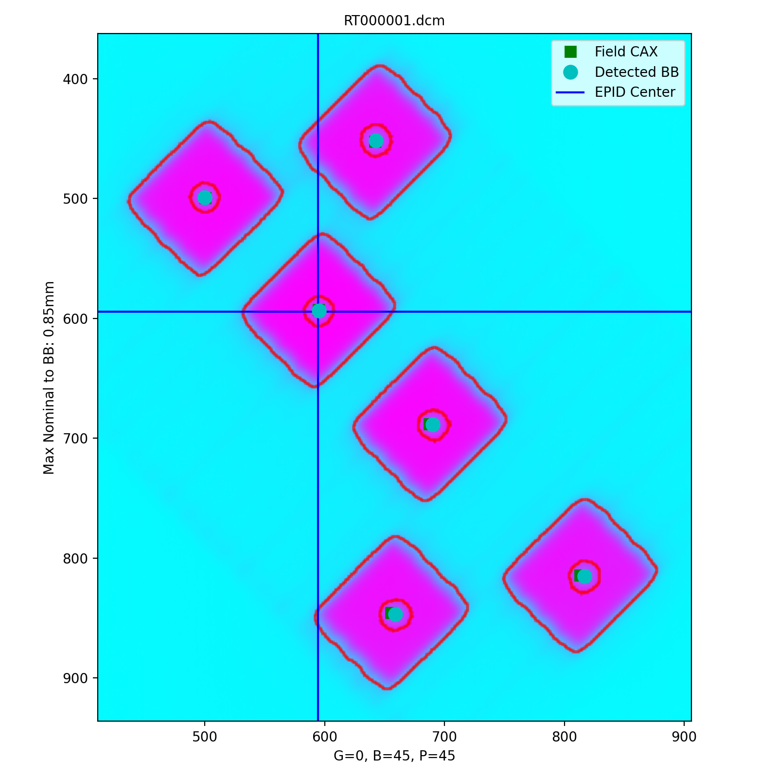
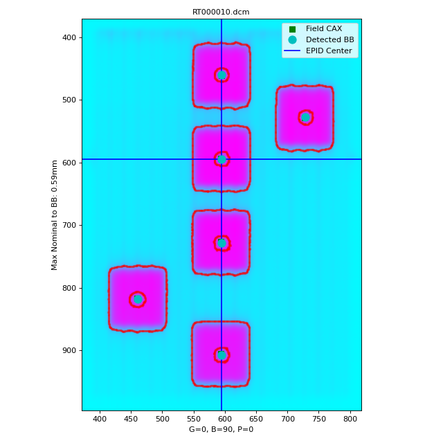
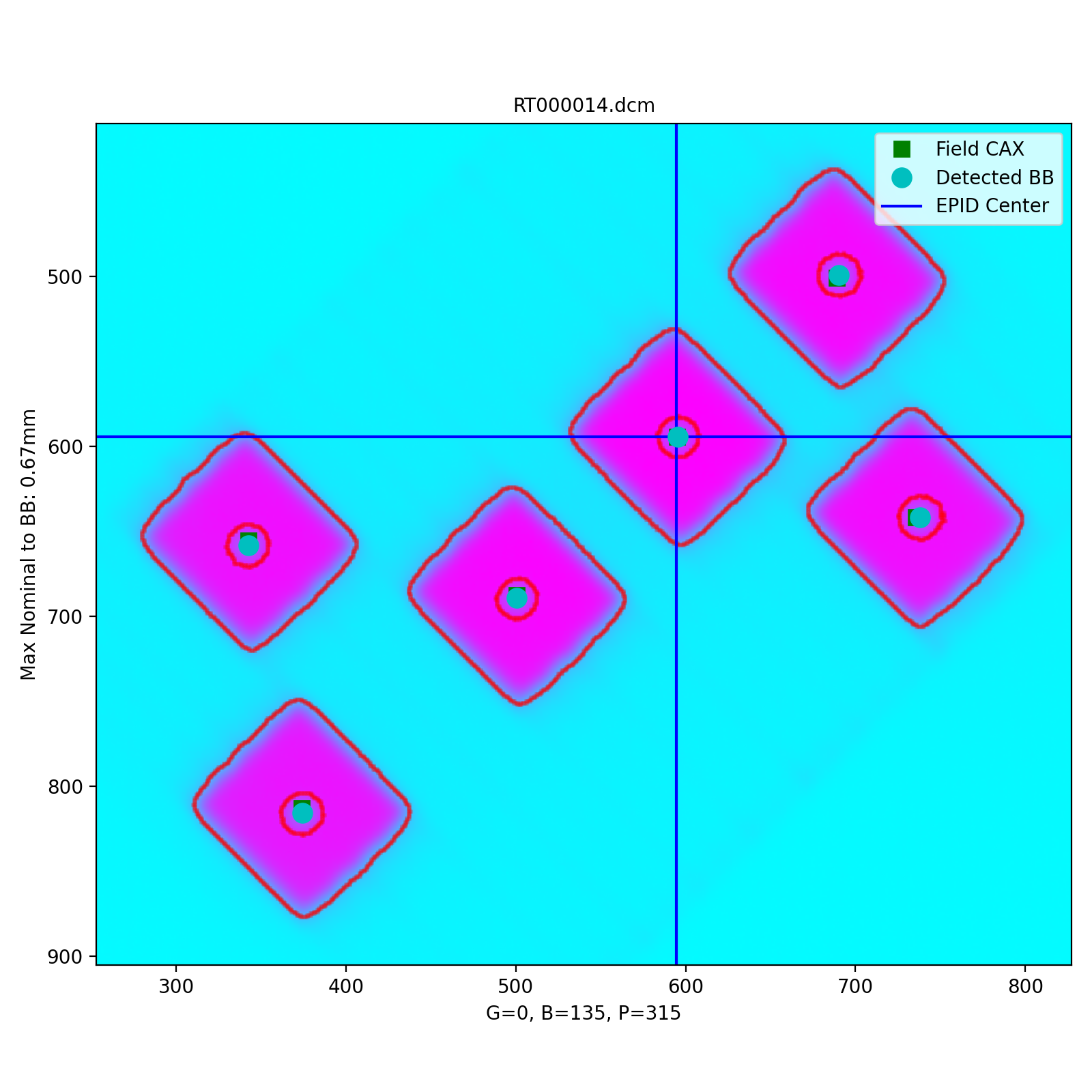
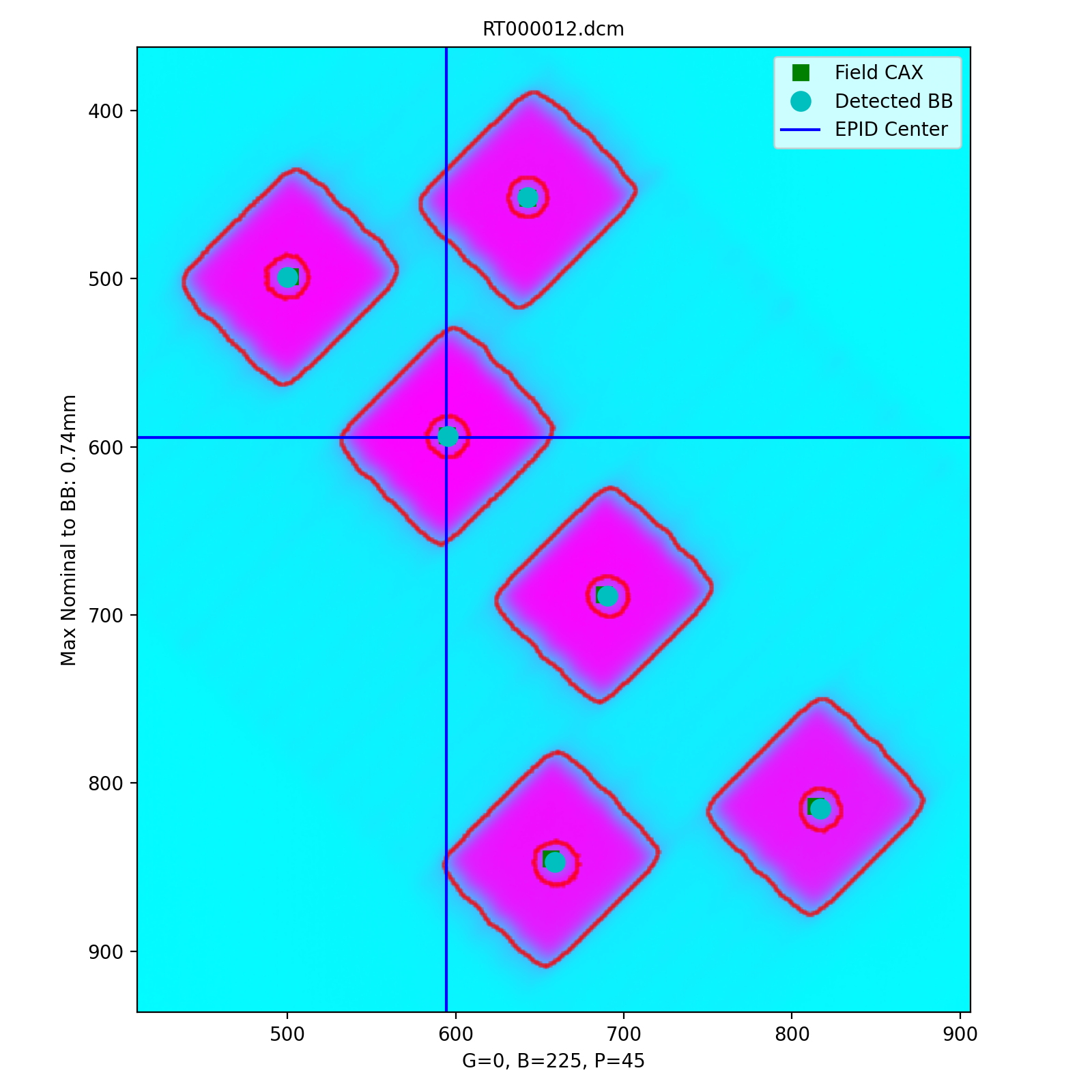
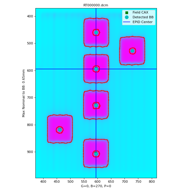
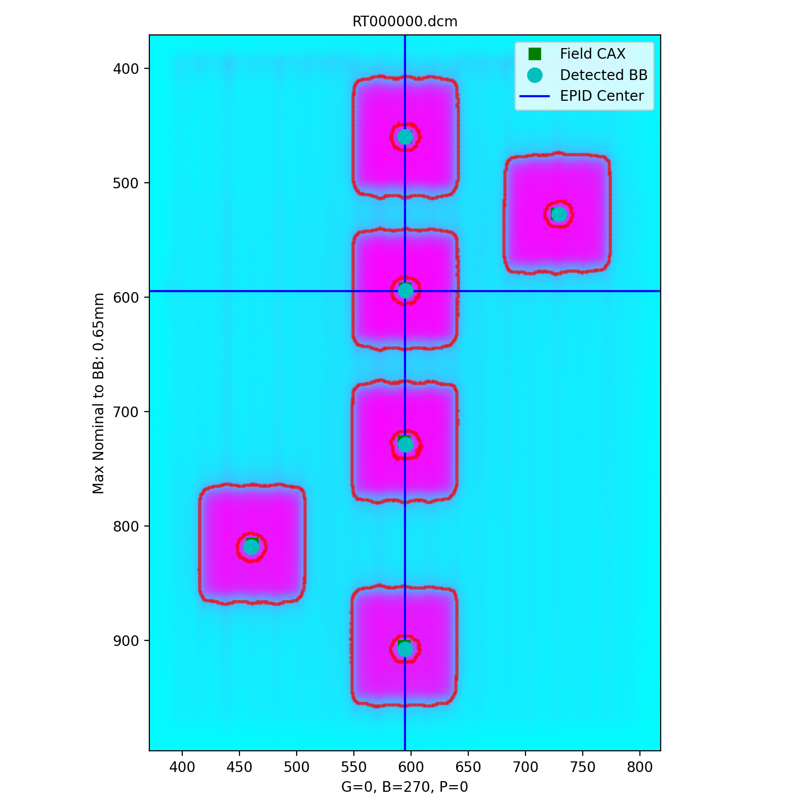
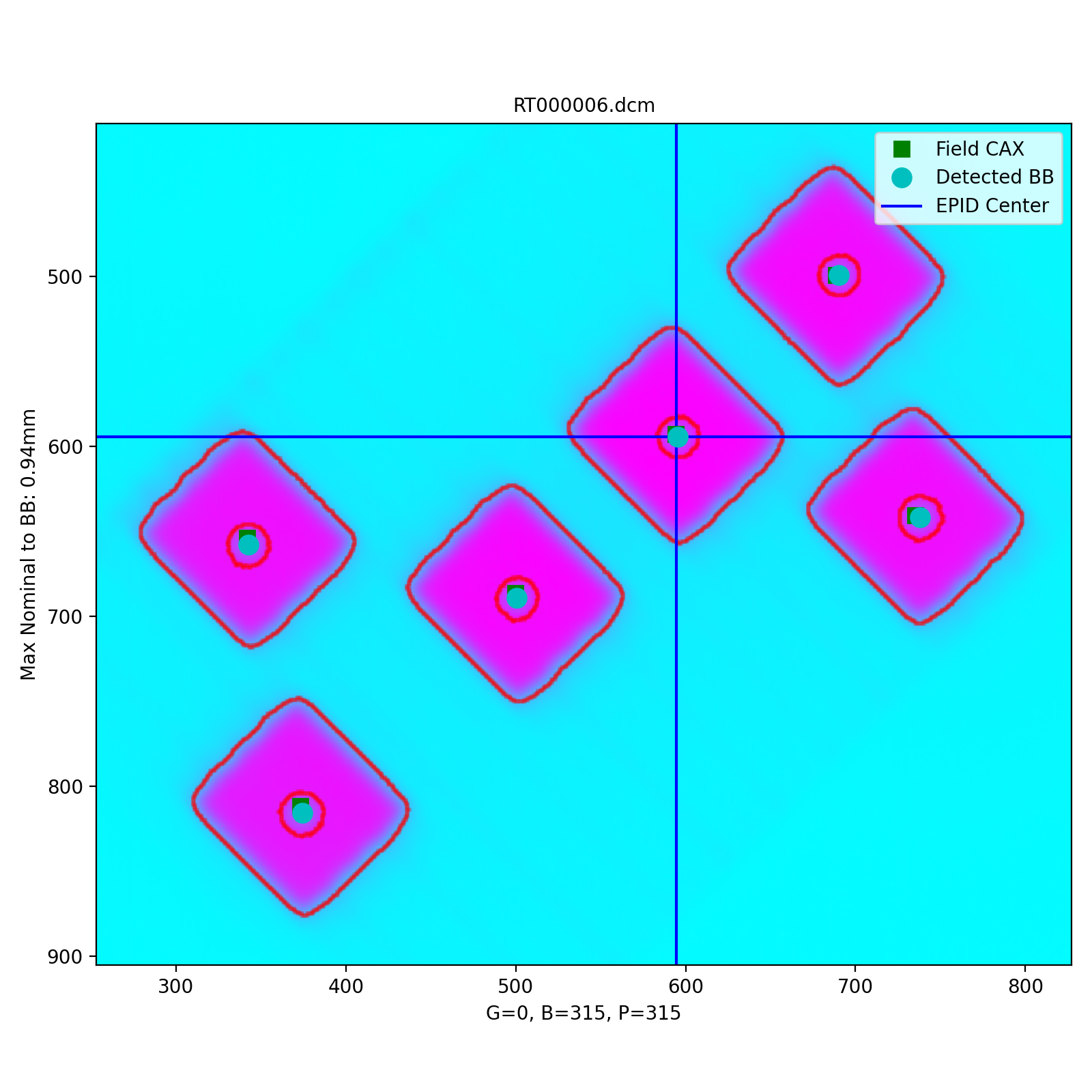
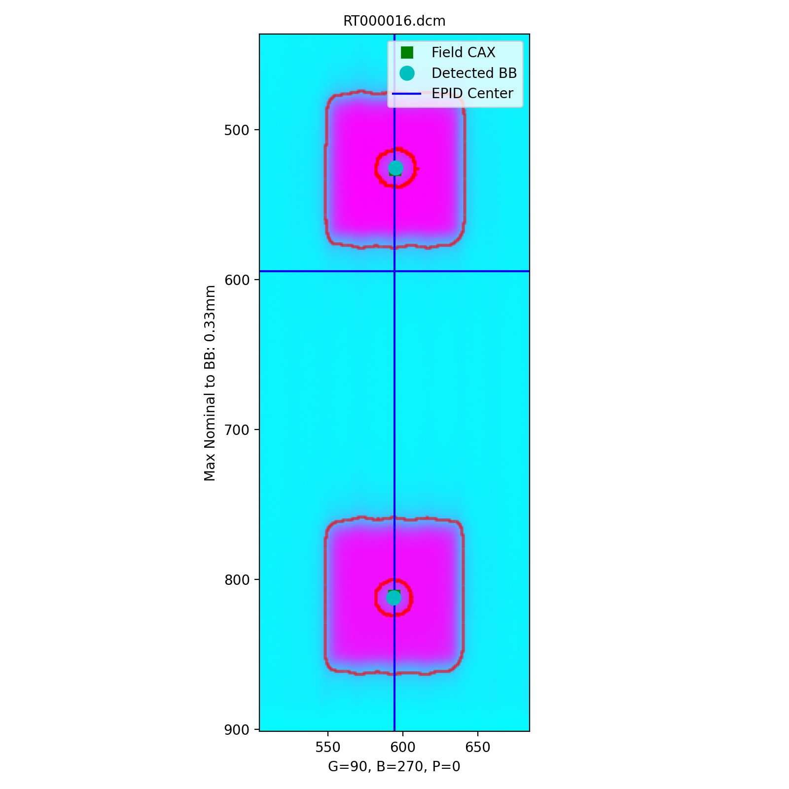
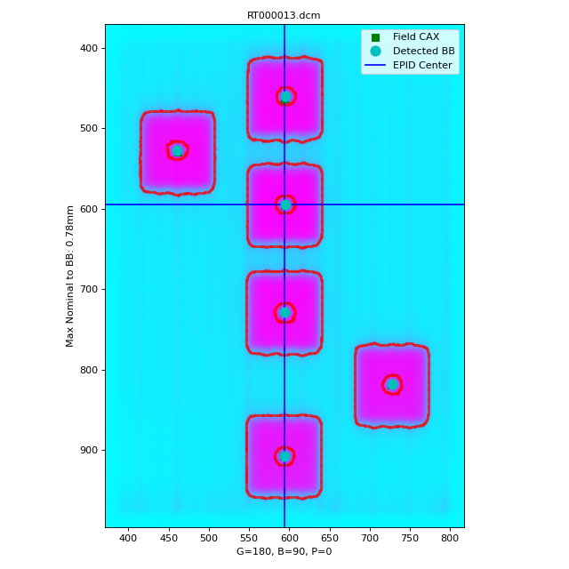
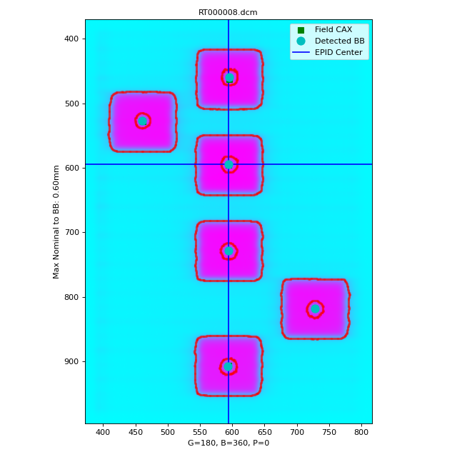
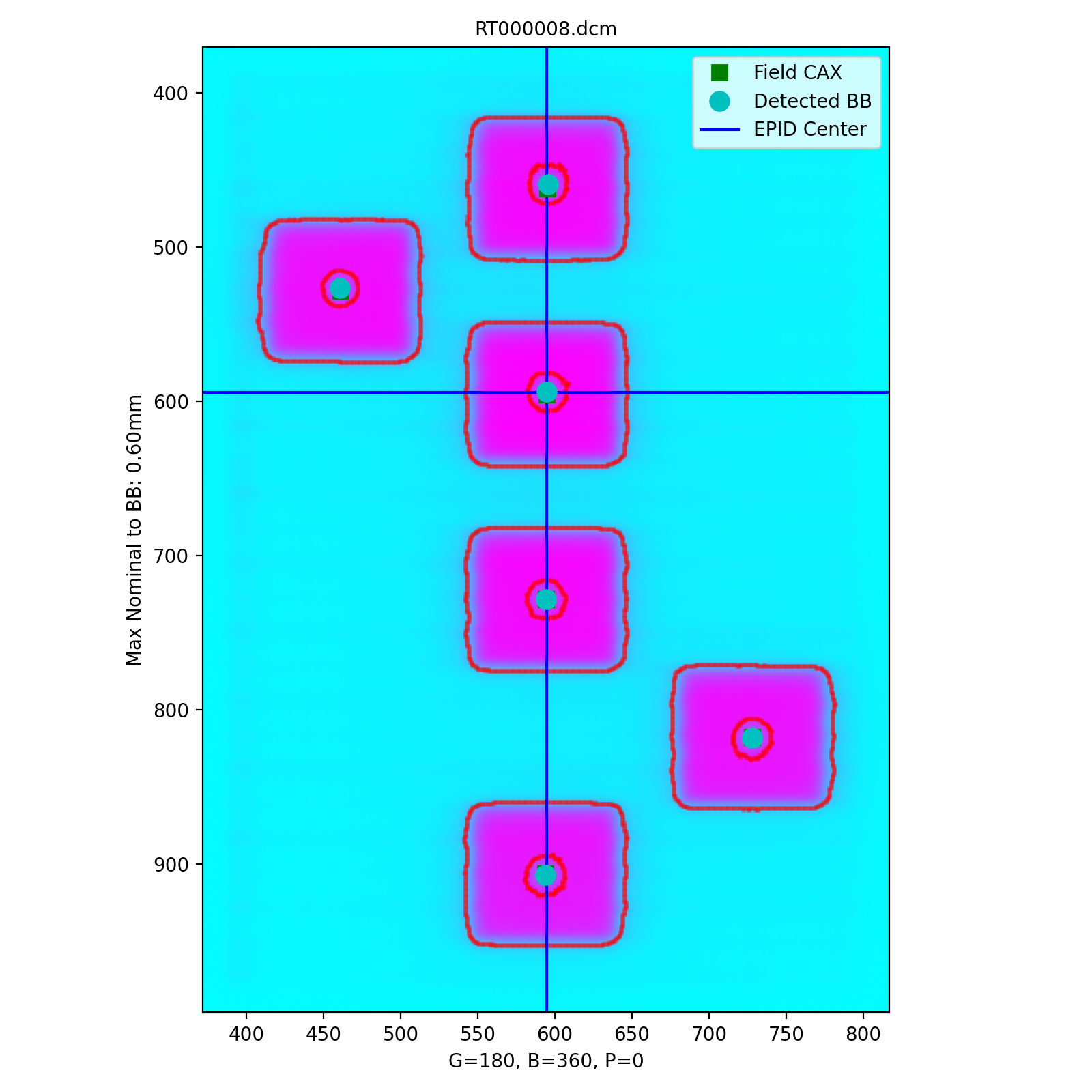
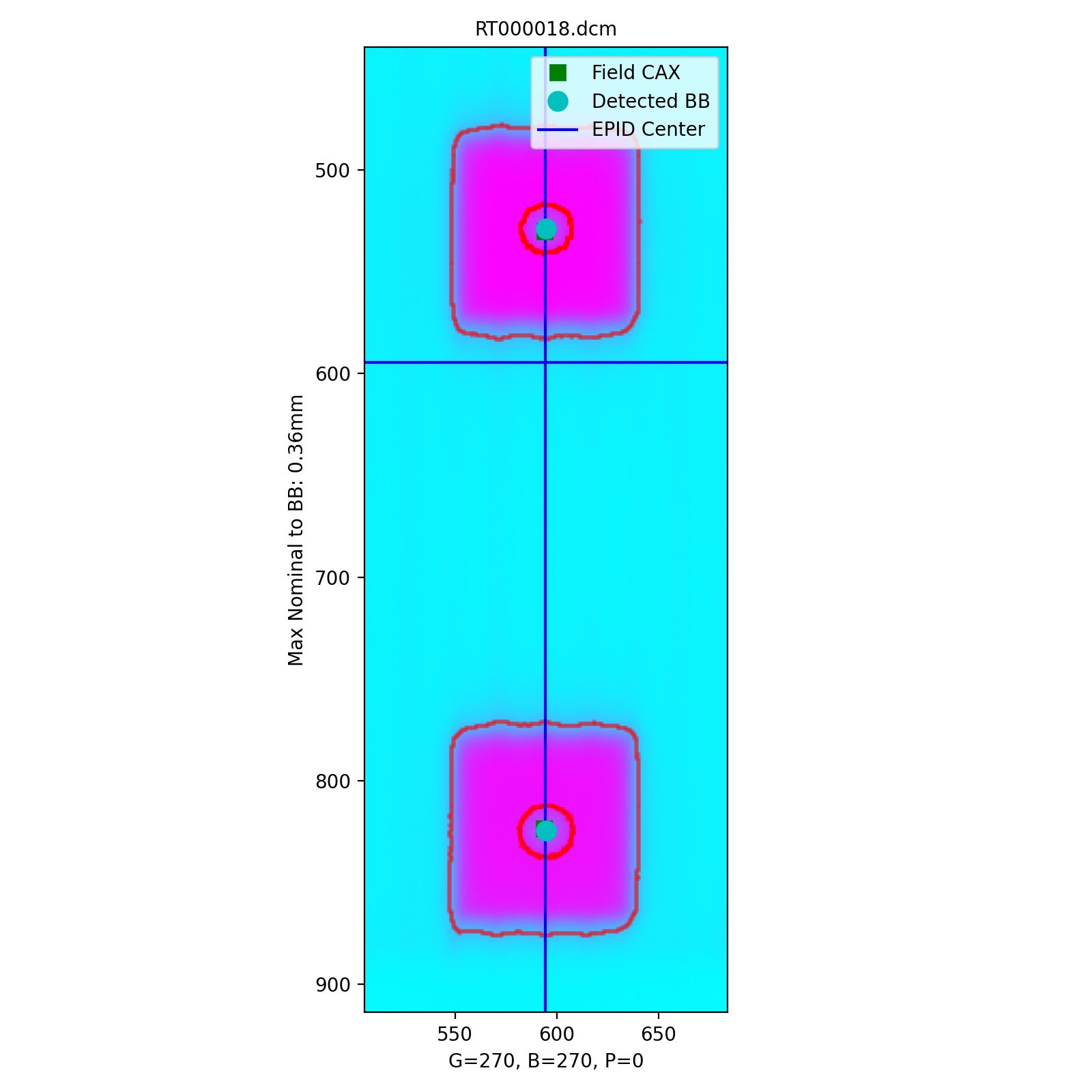
Results will be printed to the console and a figure showing the zoomed-in images will be generated:
Winston-Lutz Multi-Target Multi-Field Analysis
==============================================
Number of images: 19
2D distances
============
Max 2D distance of any BB->Field: 0.94 mm
Mean 2D distance of any BB->Field: 0.41 mm
Median 2D distance of any BB->Field: 0.37 mm
BB # Description
------ ---------------------------------
Iso Left 0.0mm, Up 0.0mm, In 0.0mm
1 Left 0.0mm, Up 0.0mm, In 30.0mm
2 Right 30.0mm, Up 0.0mm, In 15.0mm
3 Left 0.0mm, Up 0.0mm, Out 30.0mm
4 Left 30.0mm, Up 0.0mm, Out 50.0mm
5 Left 0.0mm, Up 0.0mm, Out 70.0mm
Image G C P Iso 1 2 3 4 5
------------ --- --- --- ----- ---- ---- ---- ---- ----
RT000001.dcm 0 45 45 0.21 0.11 0.26 0.67 0.85 0.84
RT000010.dcm 0 90 0 0.30 0.29 0.44 0.57 0.26 0.59
RT000014.dcm 0 135 315 0.13 0.44 0.52 0.38 0.58 0.67
RT000012.dcm 0 225 45 0.14 0.32 0.16 0.50 0.74 0.67
RT000000.dcm 0 270 0 0.37 0.07 0.33 0.65 0.65 0.64
RT000006.dcm 0 315 315 0.44 0.40 0.63 0.71 0.93 0.94
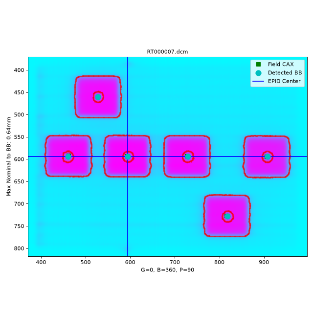
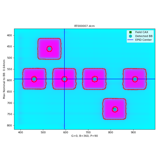
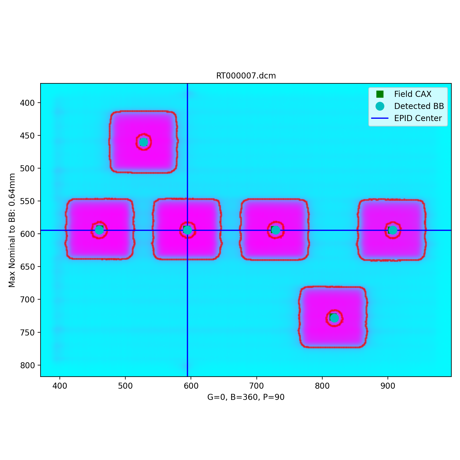
RT000007.dcm 0 360 90 0.42 0.46 0.08 0.45 0.64 0.47
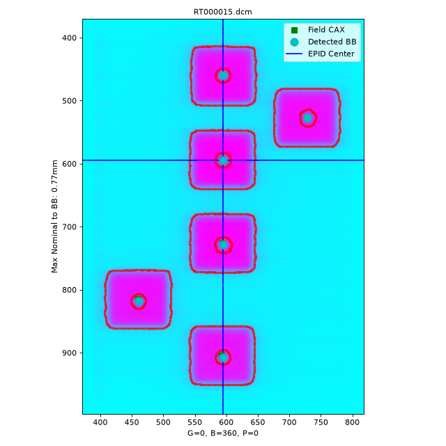
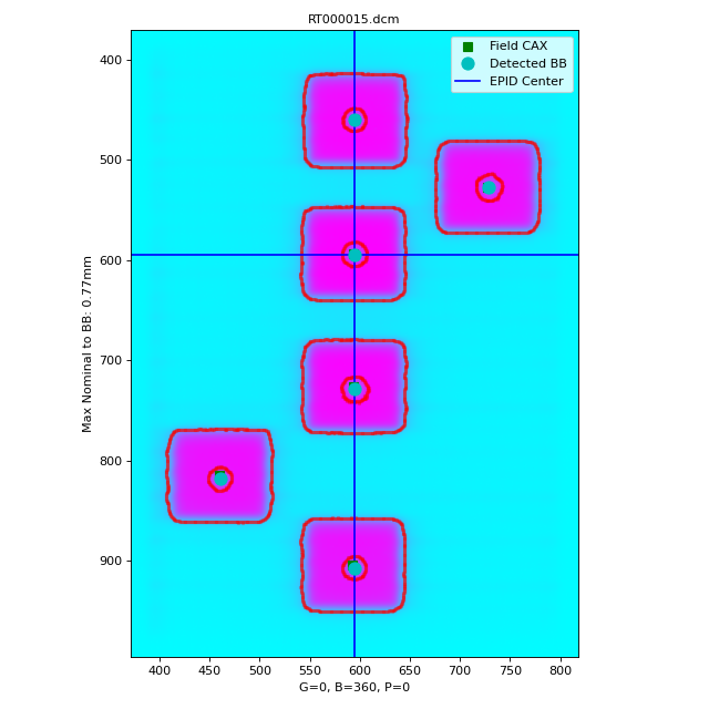
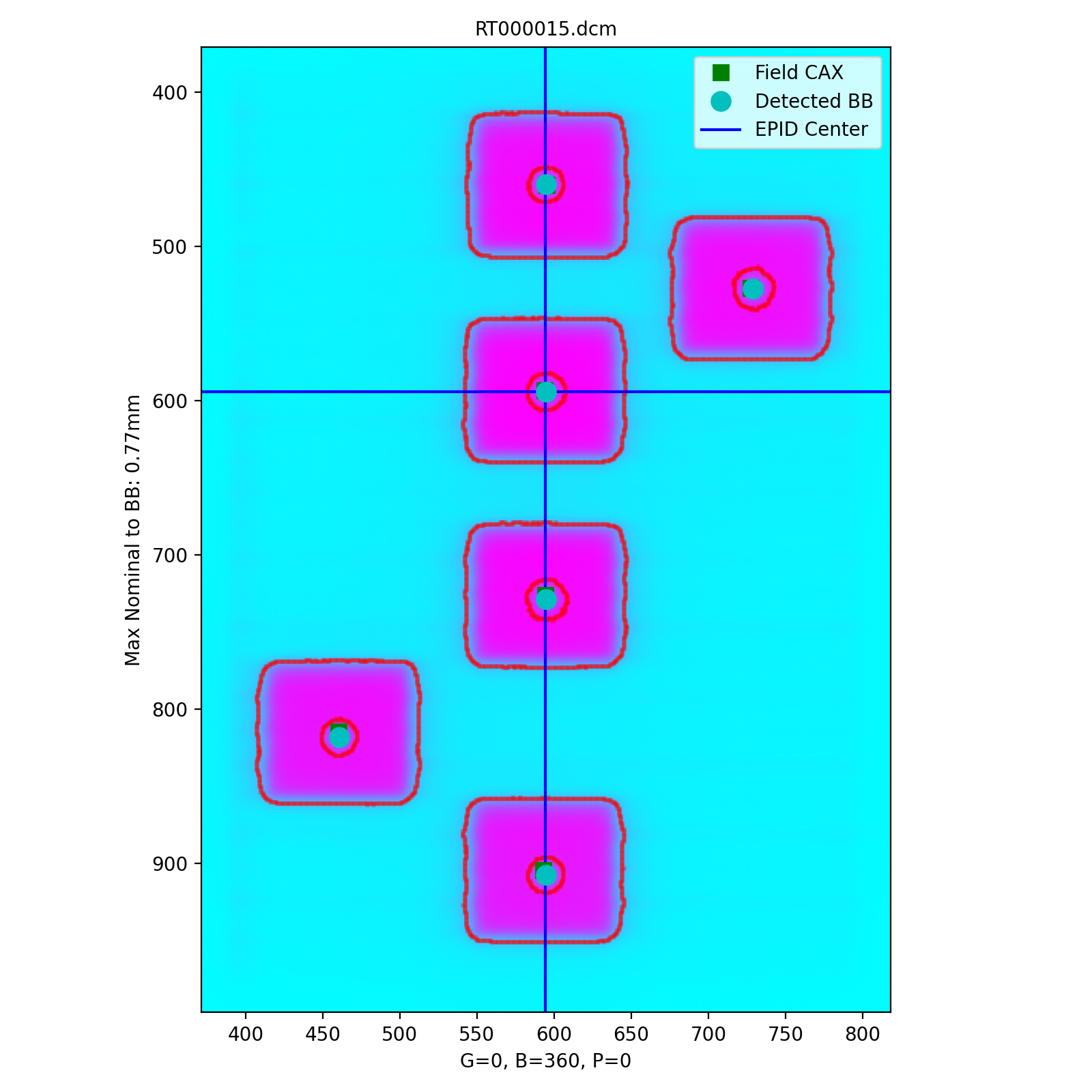
RT000015.dcm 0 360 0 0.33 0.15 0.34 0.59 0.77 0.77
RT000005.dcm 0 360 270 0.25 0.59 0.72 0.40 0.14 0.50
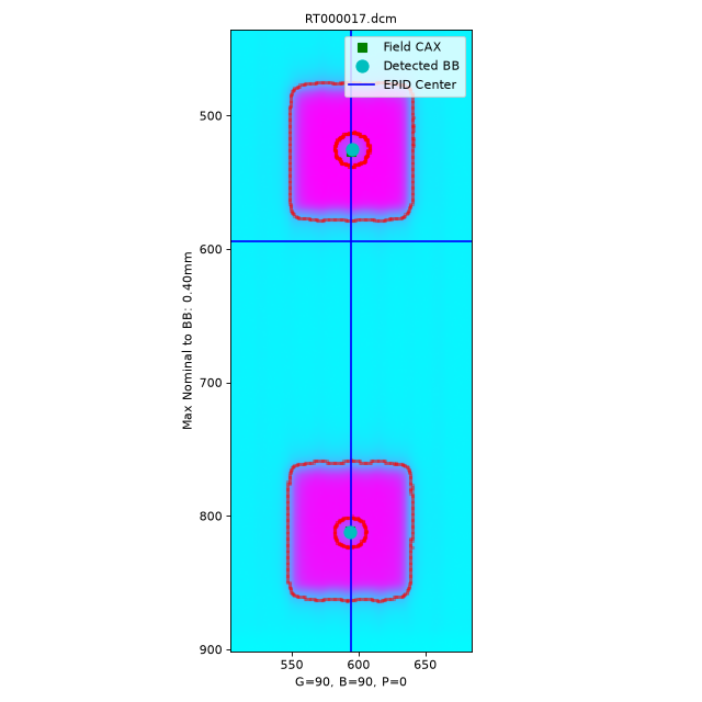
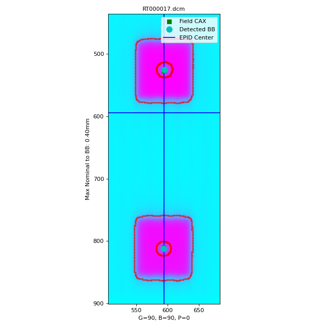
RT000017.dcm 90 90 0 --- --- 0.40 --- 0.26 ---
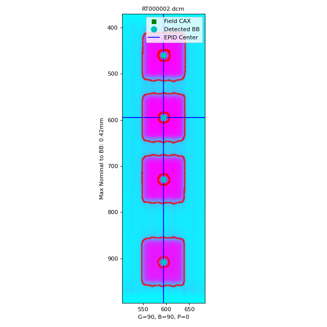
RT000002.dcm 90 90 0 0.10 0.42 --- 0.23 --- 0.22
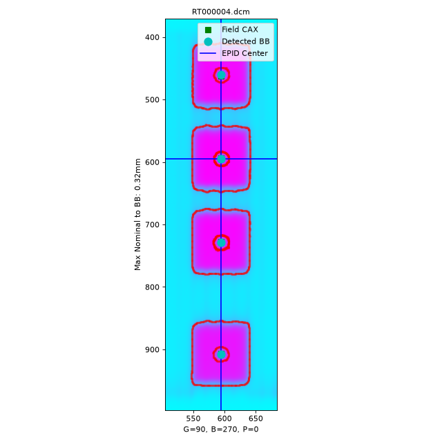
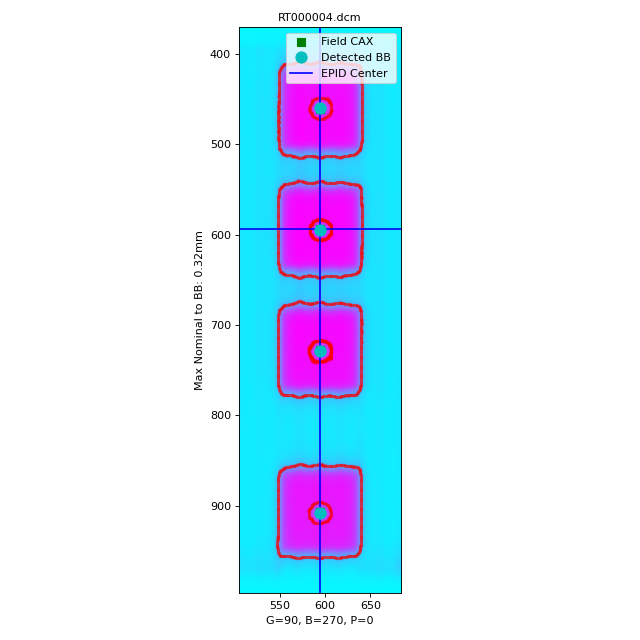
RT000004.dcm 90 270 0 0.10 0.32 --- 0.29 --- 0.27
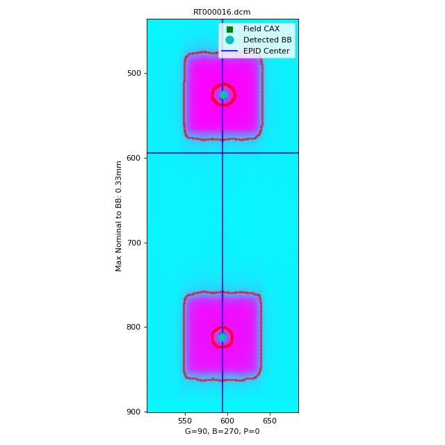
RT000016.dcm 90 270 0 --- --- 0.31 --- 0.33 ---
RT000013.dcm 180 90 0 0.33 0.78 0.58 0.19 0.32 0.24
RT000008.dcm 180 360 0 0.33 0.60 0.41 0.06 0.14 0.15
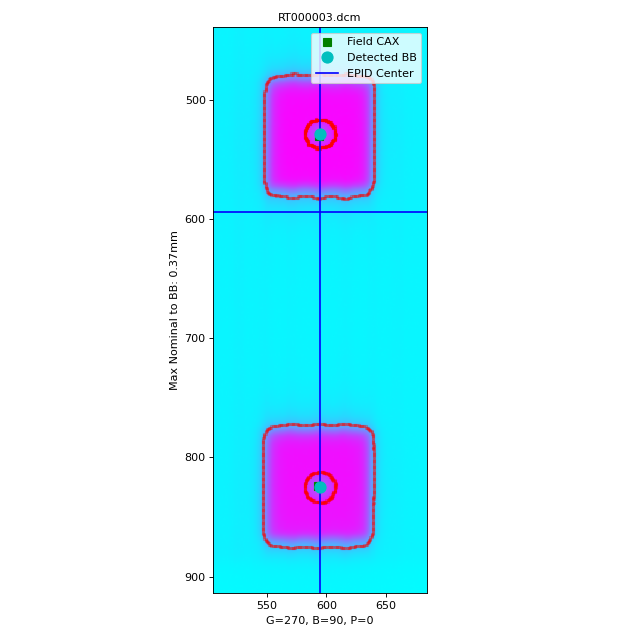
RT000003.dcm 270 90 0 --- --- 0.37 --- 0.36 ---
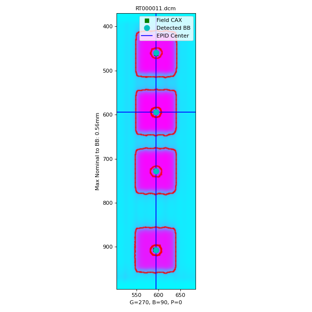
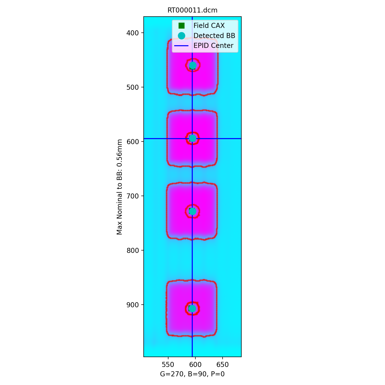
RT000011.dcm 270 90 0 0.20 0.56 --- 0.30 --- 0.37
RT000009.dcm 270 270 0 0.22 0.44 --- 0.33 --- 0.42
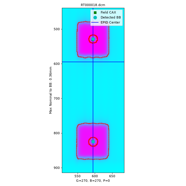
RT000018.dcm 270 270 0 --- --- 0.36 --- 0.33 ---
Image Couch Angle Yaw Error (°)
------------ ------------- ---------------
RT000007.dcm 89.998 0.12
RT000015.dcm 0.00195312 0.21
RT000005.dcm 270.002 0.25


Image Acquisition
The Winston-Lutz module will only load EPID images. The images can be from any EPID however and any SID. To ensure the most accurate results the following should be noted:
The BBs should not occlude each other.
The BBs should be >10mm apart in any given image by default.
Not all BBs must be seen in all images; i.e. some BBs can be hidden.
The radiation fields should have >5mm separation in any given image.
Coordinate Space
The MTWL algorithm uses the same coordinate system as the vanilla WL. Coordinate Space.
Passing a coordinate system
No coordinate system is passed or used (yet).
Note
This is a target for the MTWL algorithm, so expect this to change in the future.
Supported Phantoms
Currently, only the MultiMet-WL cube from SNC is supported. However, the algorithm is generalized and can be easily adapted to analyze other phantoms. See Custom BB Arrangements.
Typical Use
Analyzing a multi-target Winston-Lutz test is simple. First, let’s import the class:
from pylinac import WinstonLutzMultiTargetMultiField
from pylinac.winston_lutz import BBArrangement
From here, you can load a directory:
my_directory = "path/to/wl_images"
wl = WinstonLutzMultiTargetMultiField(my_directory)
You can also load a ZIP archive with the images in it:
wl = WinstonLutzMultiTargetMultiField.from_zip("path/to/wl.zip")
Now, analyze it. Unlike the vanilla WL algorithm, we have to pass the BB arrangement to know where the BBs should be in space. Preset phantoms exist, or a custom arrangement can be passed.
wl.analyze(bb_arrangement=BBArrangement.SNC_MULTIMET)
And that’s it! You can now view images, print the results, or publish a PDF report:
# plot all the images
wl.plot_images()
# save figures of the image plots for each bb
wl.save_images(prefix="snc")
# print to PDF
wl.publish_pdf("mymtwl.pdf")
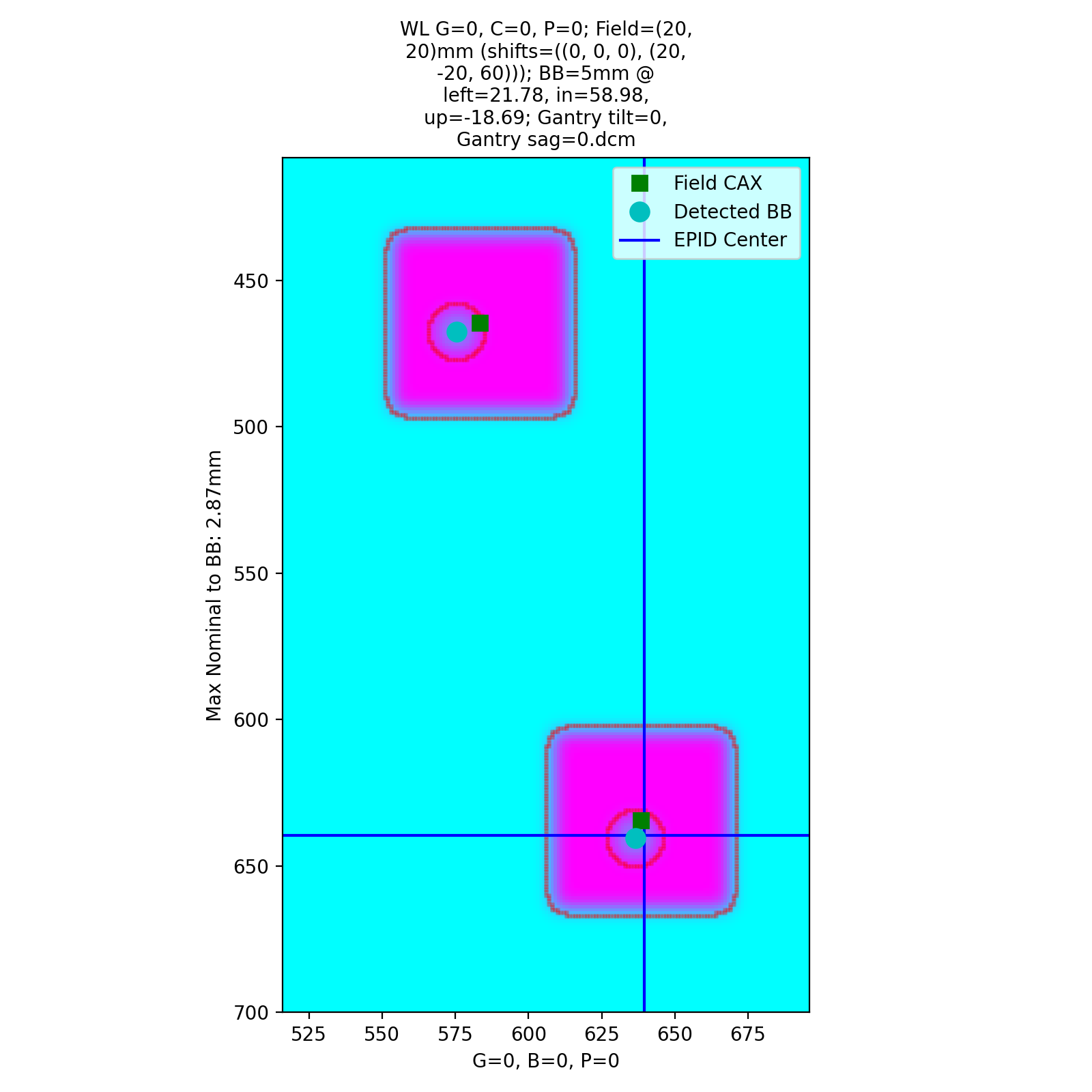
Visualizing BBs in space
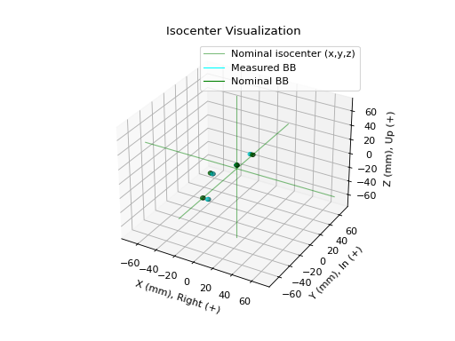
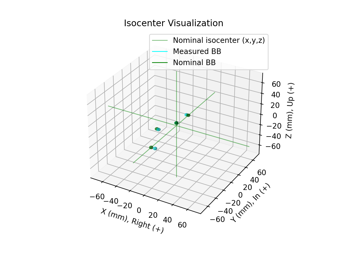
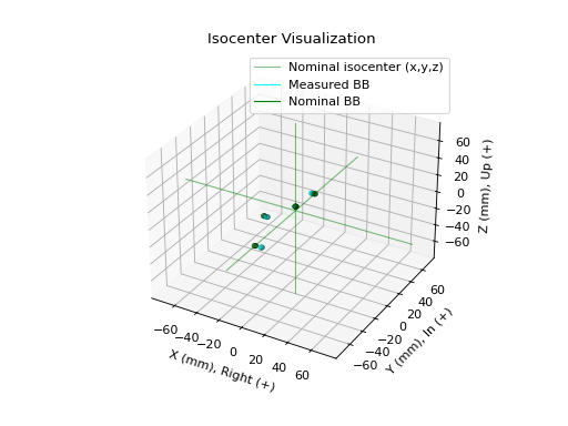
The BBs can be visualized by using the plot_location() method
and will show all the measured BB locations and their nominal locations.
(Source code, png, hires.png, pdf)
Changing BB detection size
To change the size of BB pylinac is expecting you must change it in the BB arrangement. This allows phantoms with multiple BB sizes to still be analyzed. See Custom BB Arrangements
Custom BB Arrangements
Note
Changed in version 3.22.
The BB arrangement was changed to a be a class instance instead of a simple dictionary. See BBConfig.
The MTWL algorithm uses a priori BB arrangements. I.e. you need to know where the BBs should exist in space relative to isocenter. The MTWL algorithm is flexible to accommodate any reasonable arrangement of BBs.
To create a custom arrangement, say for an in-house phantom or commercial phantom not yet supported, define the BB offsets and size like so. Use negative values to move the other direction:
from pylinac.winston_lutz import BBConfig

my_special_phantom_bbs = [
    BBConfig(
        name="Iso",
        offset_left_mm=0,
        offset_up_mm=0,
        offset_in_mm=0,
        bb_size_mm=5,
        rad_size_mm=20,
    ),  # 5mm BB at iso
    BBConfig(
        name="Left",
        offset_left_mm=30,
        offset_up_mm=0,
        offset_in_mm=0,
        bb_size_mm=4,
        rad_size_mm=20,
    ),  # 4mm BB 30mm to left of iso
    BBConfig(
        name="Down and In",
        offset_left_mm=0,
        offset_up_mm=-20,
        offset_in_mm=10,
        bb_size_mm=5,
        rad_size_mm=20,
    ),  # BB DOWN 20mm and in 10mm
    # keep going as needed
]
Pass it to the algorithm like so:
wl = WinstonLutzMultiTargetMultiField(...)
wl.analyze(bb_arrangement=my_special_phantom_bbs)
...
Analysis Parameters
See analyze() for details.
There are no specific parameters for the MTWL algorithm in RadMachine. RadMachine’s analysis is specifically for the SNC MultiMet phantom, which has known BB positions and field sizes and placements.
Algorithm
The MTWL algorithm is based on the vanilla WL algorithm. For each BB and image combination, the image is searched at the nominal location for the BB and radiation field. If it’s not found it will be skipped for that combo. The BB must be detected in at least one image or an error will be raised.
The algorithm works like such:
Allowances
The images can be acquired with any EPID (aS500, aS1000, aS1200) at any SID.
The image can have any number of BBs.
The BBs can be at any 3D location.
Restrictions
Warning
Analysis can fail or give unreliable results if any Restriction is violated.
BBs must not occlude or be <5 mm from each other in any 2D image.
The radiation fields should have >5mm separation in any given image.
Analysis
This algorithm is performed for each BB and image combination:
Find the field center – The spread in pixel values (max - min) is divided by 2, and any pixels above the threshold is associated with the open field. The pixels are converted to black & white and the center of mass of the pixels is assumed to be the field center.
Find the BB – The image is converted to binary based on pixel values both above the 50% threshold as above, and below the upper threshold. The upper threshold is an iterative value, starting at the image maximum value, that is lowered slightly when the BB is not found. If the binary image has a reasonably circular ROI, is approximately the right size, and is within 5mm of the expected BB position, the BB is considered found and the pixel-weighted center of mass of the BB is considered the BB location.
Evaluate against the field position – Once the measured BB and field positions are known, both the scalar distance and vector from the field position to the measured BB position is determined.
Interpreting Results
The results in RadMachine and those from calling results_data are as follows:
num_total_images: The total number of images analyzed.max_2d_field_to_bb_mm: The maximum 2D distance from any BB to its field center.median_2d_field_to_bb_mm: The median 2D distance from any BB to its field center.mean_2d_field_to_bb_mm: The mean 2D distance from any BB to its field center.bb_arrangement: A list of the nominal locations of the BBs. Each BB arrangement has the following items:name: The name of the BB.offset_left_mm: The offset in the left-right direction from isocenter. See: Coordinate Space.offset_up_mm: The offset in the up-down direction from isocenter.offset_in_mm: The offset in the in-out direction from isocenter.bb_size_mm: The size of the BB in mm.rad_size_mm: The size of the radiation field in mm.
bb_maxes: A dictionary of the maximum 2D distances of each BB to its field center. The key is the BB name as defined in the arrangement.bb_shift_vector: The vector (in 3D cartesian space) to move the phantom to align with the isocenter in mm.bb_shift_yaw: The yaw rotation in degrees needed to align the phantom with the radiation isocenter.bb_shift_pitch: The pitch rotation needed in degrees to align the phantom with the radiation isocenter.bb_shift_roll: The roll rotation needed in degrees to align the phantom with the radiation isocenter.
Benchmarking the Algorithm
With the image generator module we can create test images to test the WL algorithm on known results. This is useful to isolate what is or isn’t working if the algorithm doesn’t work on a given image and when commissioning pylinac. It is common, especially with the WL module, to question the accuracy of the algorithm. Since no linac is perfect and the results are sub-millimeter, discerning what is true error vs algorithmic error can be difficult. The image generator module is a perfect solution since it can remove or reproduce the former error.
Note
With the introduction of the MTWL algorithm, so too a multi-target synthetic image generator has been created: generate_winstonlutz_multi_bb_multi_field().
Warning
The image generator is limited in accuracy to ~1/2 pixel because creating the image requires a row or column to be set. E.g. a 5mm field with a 0.336mm pixel size means we need to create a field of 14.88 pixels wide. We can only set the field to be 14 or 15 pixels, so the nearest field size of 15 pixels or 5.04mm is set.
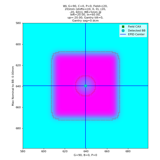
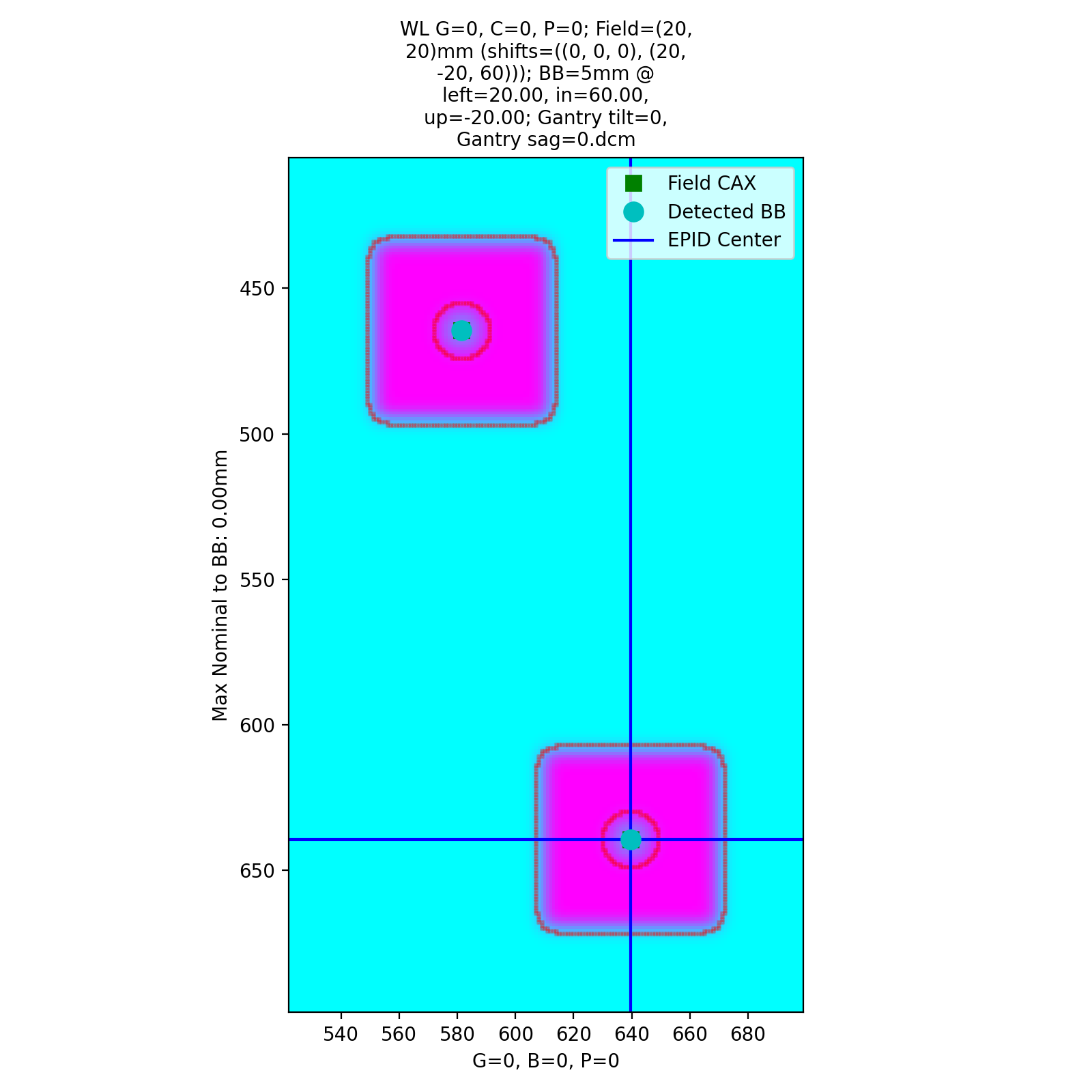
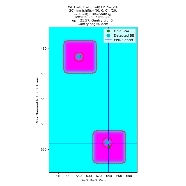
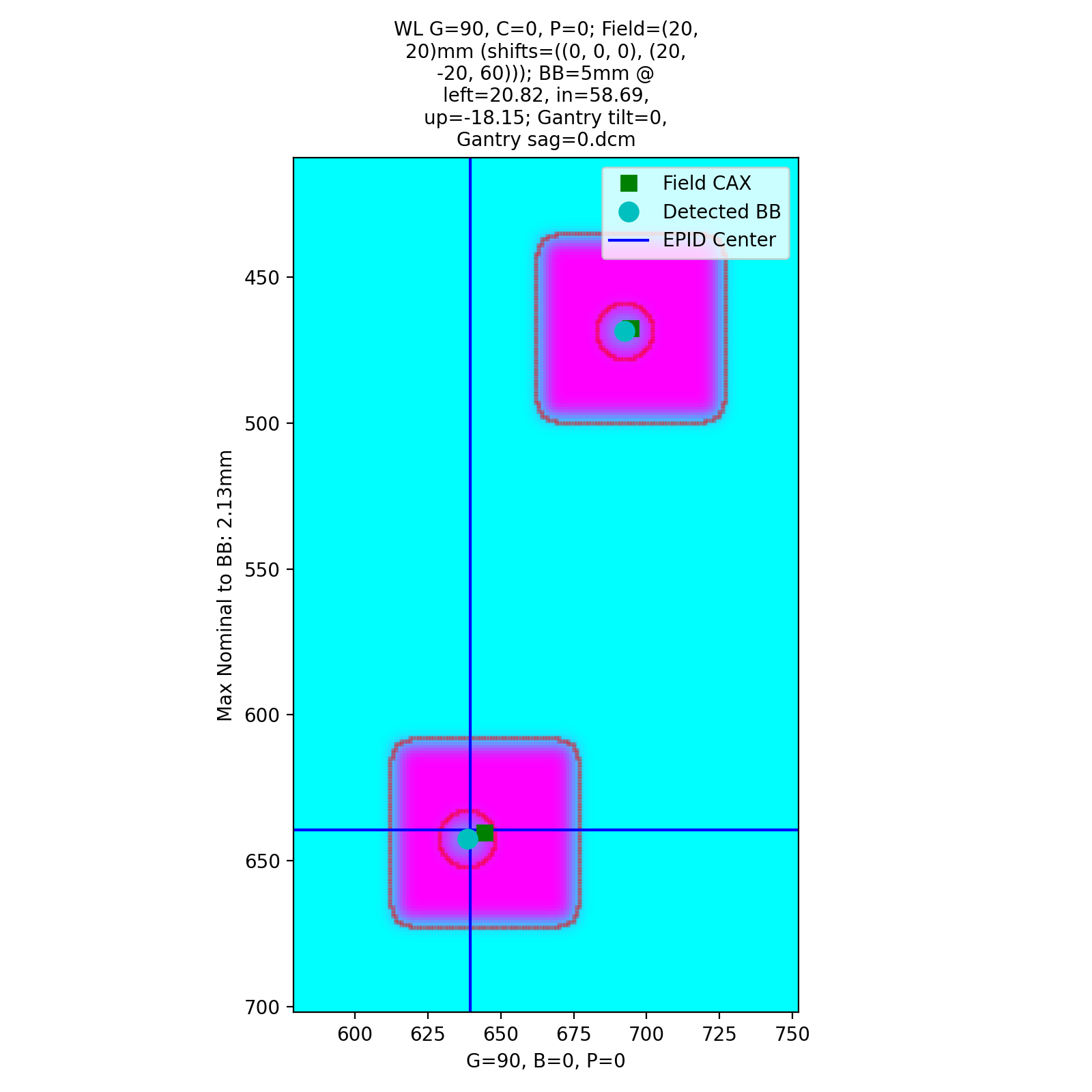
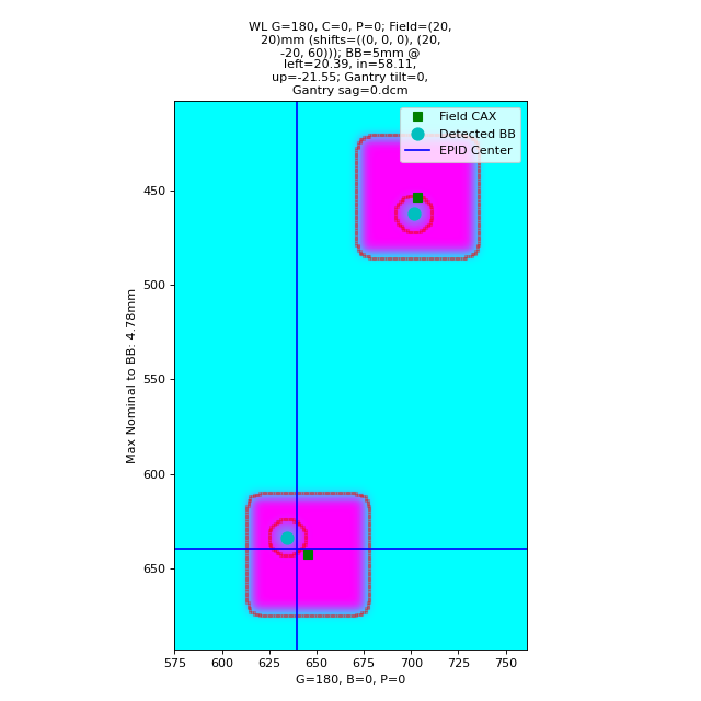
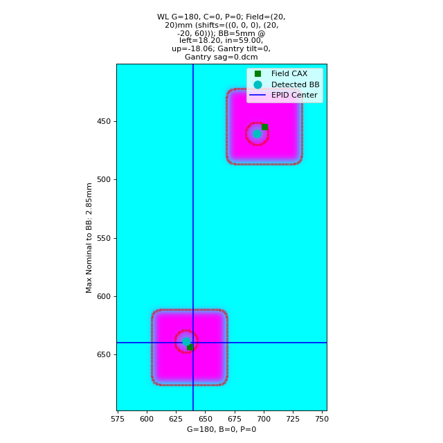
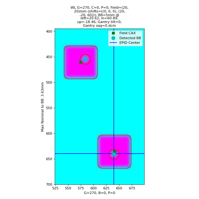
2-BB Perfect Delivery
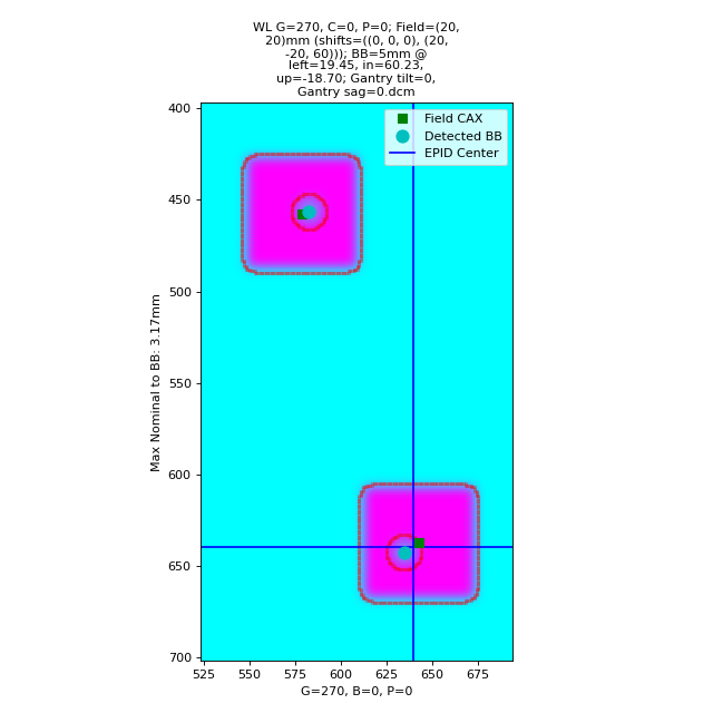
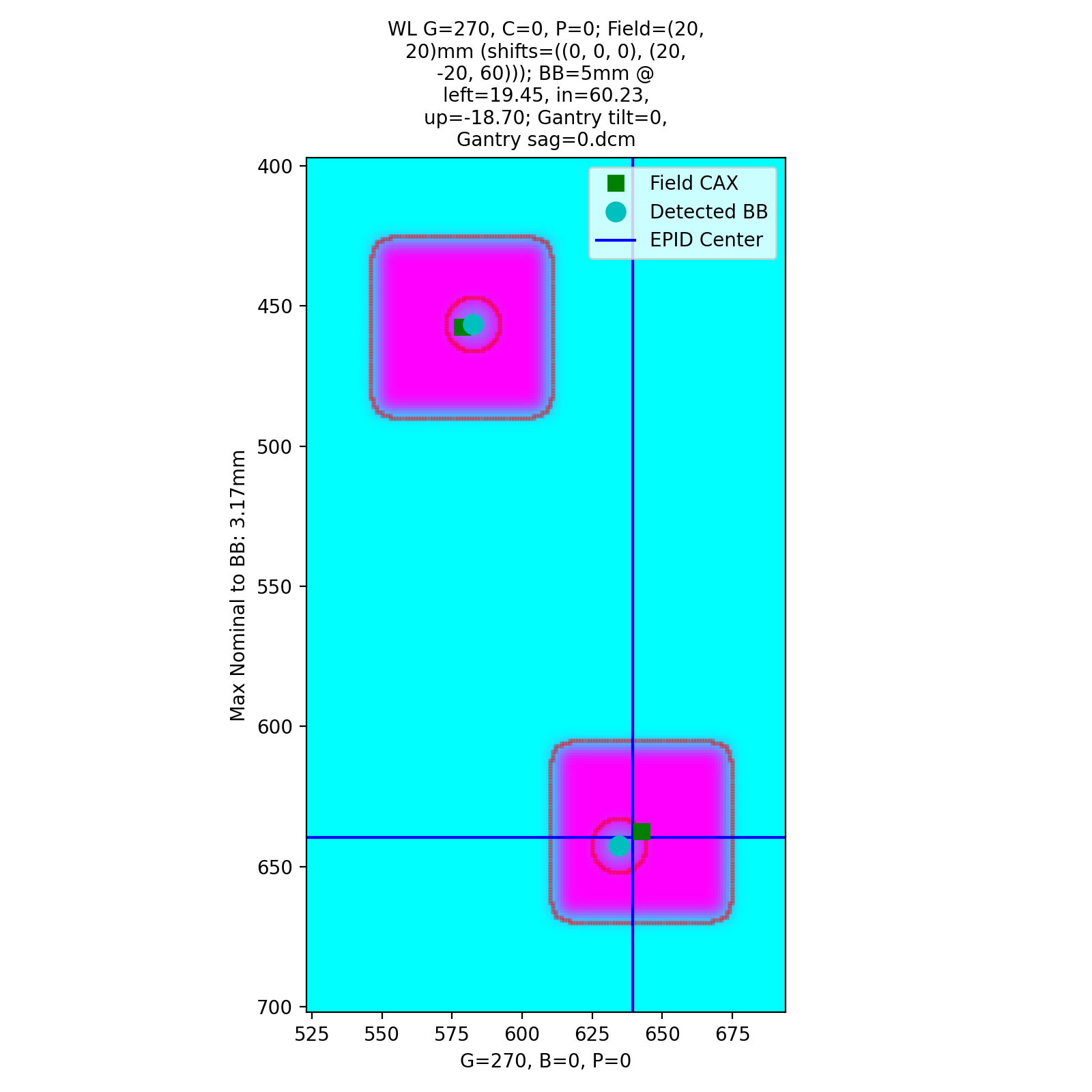
Create a perfect set of fields with 1 BB at iso and another 20mm left, 20mm down, and 60mm inward (this is the same as the demo, but is good for explanation).
import pylinac
from pylinac.winston_lutz import BBConfig
from pylinac.core.image_generator import simulators, layers, generate_winstonlutz_multi_bb_multi_field

wl_dir = 'wl_dir'
generate_winstonlutz_multi_bb_multi_field(
        simulator=simulators.AS1200Image(sid=1000),
        field_layer=layers.PerfectFieldLayer,
        final_layers=[layers.GaussianFilterLayer(sigma_mm=1),],
        dir_out=wl_dir,
        field_offsets=((0, 0, 0), (20, -20, 60)),
        field_size_mm=(20, 20),
        bb_offsets=[[0, 0, 0], [20, -20, 60]],
)
arrange = (
    BBConfig(name='Iso', offset_left_mm=0, offset_up_mm=0, offset_in_mm=0, bb_size_mm=5, rad_size_mm=20),
    BBConfig(name='Left,Down,In', offset_left_mm=20, offset_up_mm=-20, offset_in_mm=60, bb_size_mm=5, rad_size_mm=20),
)

wl = pylinac.WinstonLutzMultiTargetMultiField(wl_dir)
wl.analyze(bb_arrangement=arrange)
print(wl.results())
wl.plot_images()


which has an output of:
Winston-Lutz Multi-Target Multi-Field Analysis
==============================================
Number of images: 4

2D distances
============
Max 2D distance of any BB->Field: 0.00 mm
Mean 2D distance of any BB->Field: 0.00 mm
Median 2D distance of any BB->Field: 0.00 mm

BB #          Description
------------  -----------------------------
Iso           Left 0mm, Up 0mm, In 0mm
Left,Down,In  Left 20mm, Down 20mm, In 60mm

Image                   G    C    P    Iso    Left,Down,In
--------------------  ---  ---  ---  -----  --------------
=0, Gantry sag=0.dcm    0    0    0      0               0
=0, Gantry sag=0.dcm   90    0    0      0               0
=0, Gantry sag=0.dcm  180    0    0      0               0
=0, Gantry sag=0.dcm  270    0    0      0               0
As shown, we have perfect results.
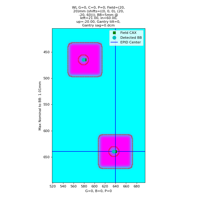
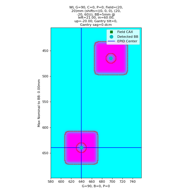
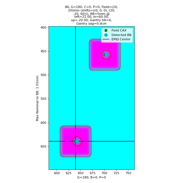
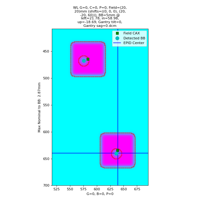
Offset BBs
Let’s now offset both BBs by 1mm to the left:
import pylinac
from pylinac.winston_lutz import BBConfig
from pylinac.core.image_generator import simulators, layers, generate_winstonlutz_multi_bb_multi_field

wl_dir = 'wl_dir'
generate_winstonlutz_multi_bb_multi_field(
        simulator=simulators.AS1200Image(sid=1000),
        field_layer=layers.PerfectFieldLayer,
        final_layers=[layers.GaussianFilterLayer(sigma_mm=1),],
        dir_out=wl_dir,
        field_offsets=((0, 0, 0), (20, -20, 60)),
        field_size_mm=(20, 20),
        bb_offsets=[[1, 0, 0], [21, -20, 60]],  # here's the offset
)
arrange = (
    BBConfig(name='Iso', offset_left_mm=0, offset_up_mm=0, offset_in_mm=0, bb_size_mm=5, rad_size_mm=20),
    BBConfig(name='Left,Down,In', offset_left_mm=20, offset_up_mm=-20, offset_in_mm=60, bb_size_mm=5, rad_size_mm=20),
)

wl = pylinac.WinstonLutzMultiTargetMultiField(wl_dir)
wl.analyze(bb_arrangement=arrange)
print(wl.results())
wl.plot_images()


with an output of:
Winston-Lutz Multi-Target Multi-Field Analysis
==============================================
Number of images: 4

2D distances
============
Max 2D distance of any BB->Field: 1.01 mm
Mean 2D distance of any BB->Field: 0.50 mm
Median 2D distance of any BB->Field: 0.50 mm

BB #          Description
------------  -----------------------------
Iso           Left 0mm, Up 0mm, In 0mm
Left,Down,In  Left 20mm, Down 20mm, In 60mm

Image                   G    C    P    Iso    Left,Down,In
--------------------  ---  ---  ---  -----  --------------
=0, Gantry sag=0.dcm    0    0    0   1.01            1.01
=0, Gantry sag=0.dcm   90    0    0   0               0
=0, Gantry sag=0.dcm  180    0    0   1.01            1.01
=0, Gantry sag=0.dcm  270    0    0   0               0
Both BBs report a shift of 1mm. Note this is only in 0 and 180. A left shift would not be captured at 90/270.
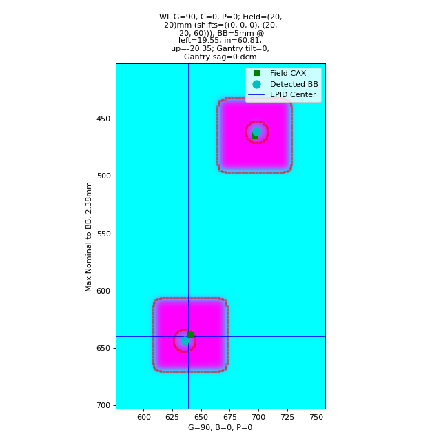
Random error
Let’s now add random error:
Note
The error is random so performing this again will change the results slightly.
import pylinac
from pylinac.winston_lutz import BBConfig
from pylinac.core.image_generator import simulators, layers, generate_winstonlutz_multi_bb_multi_field

wl_dir = 'wl_dir'
generate_winstonlutz_multi_bb_multi_field(
        simulator=simulators.AS1200Image(sid=1000),
        field_layer=layers.PerfectFieldLayer,
        final_layers=[layers.GaussianFilterLayer(sigma_mm=1),],
        dir_out=wl_dir,
        field_offsets=((0, 0, 0), (20, -20, 60)),
        field_size_mm=(20, 20),
        bb_offsets=[[0, 0, 0], [20, -20, 60]],
        jitter_mm=2  # here we add random noise
)
arrange = (
    BBConfig(name='Iso', offset_left_mm=0, offset_up_mm=0, offset_in_mm=0, bb_size_mm=5, rad_size_mm=20),
    BBConfig(name='Left,Down,In', offset_left_mm=20, offset_up_mm=-20, offset_in_mm=60, bb_size_mm=5, rad_size_mm=20),
)

wl = pylinac.WinstonLutzMultiTargetMultiField(wl_dir)
wl.analyze(bb_arrangement=arrange)
print(wl.results())
wl.plot_images()
with an output of:
Winston-Lutz Multi-Target Multi-Field Analysis
==============================================
Number of images: 4

2D distances
============
Max 2D distance of any BB->Field: 4.21 mm
Mean 2D distance of any BB->Field: 1.74 mm
Median 2D distance of any BB->Field: 1.39 mm

BB #          Description
------------  -----------------------------
Iso           Left 0mm, Up 0mm, In 0mm
Left,Down,In  Left 20mm, Down 20mm, In 60mm

Image                   G    C    P    Iso    Left,Down,In
--------------------  ---  ---  ---  -----  --------------
=0, Gantry sag=0.dcm    0    0    0   2.38            2.71
=0, Gantry sag=0.dcm   90    0    0   1.06            1.39
=0, Gantry sag=0.dcm  180    0    0   4.21            1.39
=0, Gantry sag=0.dcm  270    0    0   0.48            0.34
API Documentation
- class pylinac.winston_lutz.WinstonLutzMultiTargetMultiField(directory: str | list[str] | Path, use_filenames: bool = False, axis_mapping: dict[str, tuple[float | None, float | None, float | None]] | None = None, axes_precision: int | None = None, dpi: float | None = None, sid: float | None = None, missing_axis_value: float | Literal['raise'] = 'raise')[source]
Bases:
WinstonLutzParameters
- directorystr, list[str]
Path to the directory of the Winston-Lutz EPID images or a list of the image paths
- use_filenames: bool
Whether to try to use the file name to determine axis values. Useful for Elekta machines that do not include that info in the DICOM data. This is mutually exclusive to axis_mapping. If True, axis_mapping is ignored.
- axis_mapping: dict
An optional way of instantiating by passing each file along with the axis values. Structure should be <filename>: (<gantry>, <coll>, <couch>). Each value must be numeric.
Noneis treated as missing and will raise an error.- axes_precision: int | None
How many significant digits to represent the axes values. If None, no precision is set and the input/DICOM values are used raw. If set to an integer, rounds the axes values (gantry, coll, couch) to that many values. E.g. gantry=0.1234 => 0.1 with precision=1. This is mostly useful for plotting/rounding (359.9=>0) and if using the
keyed_image_detailswithresults_data.- dpi
The dots-per-inch setting. Only needed if using TIFF images and the images do not contain the resolution tag. An error will raise if dpi is not passed and the TIFF resolution cannot be determined.
- sid
The Source-to-Image distance in mm. Only needed when using TIFF images.
- missing_axis_value
The value to use if an axis value cannot be determined. If “raise”, an error will be raised instead. Use 0 to match the historical behavior.
- machine_scale: MachineScale
- images: Sequence[WinstonLutzMultiTargetMultiFieldImage]
- image_type
- bbs: list[BB3D]
3D representation of the BBs
- static run_demo()[source]
Run the Winston-Lutz MT MF demo, which loads the demo files, prints results, and plots a summary image.
- analyze(bb_arrangement: tuple[BBConfig, ...], is_open_field: bool = False, is_low_density: bool = False, machine_scale: MachineScale = MachineScale.IEC61217, bb_proximity_mm: float = 10)[source]
Analyze the WL images.
Parameters
- bb_arrangement
The arrangement of the BBs in the phantom. A dict with offset and BB size keys. See the
BBArrangementclass for keys and syntax.
See Also
WinstonLutz.analyze for other parameter info.
- plot_location(show: bool = True, viewbox_mm: float | None = None, plot_bb: bool = True, plot_isocenter_sphere: bool = True, plot_couch_iso: bool = True, plot_coll_iso: bool = True, show_legend: bool = True)[source]
Plot the isocenter and size as a sphere in 3D space relative to the BB. The iso is at the origin.
Only images where the couch was at zero are considered.
Parameters
- showbool
Whether to plot the image.
- viewbox_mmfloat
The default size of the 3D space to plot in mm in each axis.
- plot_bbbool
Whether to plot the BB location; the size is also considered.
- plot_isocenter_spherebool
Whether to plot the gantry + collimator isocenter size.
- plot_couch_isobool
Whether to plot the couch-plane-only isocenter size. This will be zero if there are no images where the couch rotated.
- plot_coll_isobool
Whether to plot the collimator-plane-only isocenter size. This is shown along the Z/Y plane only to differentiate from the couch iso visualization. The collimator plane is always normal to the gantry angle. This will be zero if there are no images where the collimator rotated.
- show_legendbool
Whether to show the legend.
- property bb_shift_vector: Vector, float, float, float
Calculate the ideal shift in 6 degrees of freedom to place the BB at the isocenter.
Returns
- Vector
The ideal shift vector in mm for the cartesian coordinates. X,Y, and Z follow the pylinac coordinate convention.
- float
Yaw; The ideal rotation about the Z-axis in degrees.
- float
Pitch; The ideal rotation about the X-axis in degrees.
- float
Roll; The ideal rotation about the Y-axis in degrees.
See Also
Euler Angles: https://en.wikipedia.org/wiki/Euler_angles Gimbal Lock: https://en.wikipedia.org/wiki/Gimbal_lock
- bb_shift_instructions() str[source]
Return a string that provides instructions on how to shift the BB to the isocenter.
- property gantry_coll_iso_size: float
The diameter of the 3D gantry isocenter size in mm including collimator and gantry/coll combo images. Images where the couch!=0 are excluded.
- property collimator_iso_size: float
The 2D collimator isocenter size (diameter) in mm. The iso size is in the plane normal to the gantry.
- property couch_iso_size: float
The diameter of the 2D couch isocenter size in mm. Only images where the gantry and collimator were at zero are used to determine this value.
- property gantry_iso_size: float
The diameter of the 3D gantry isocenter size in mm. Only images where the collimator and couch were at 0 are used to determine this value.
- plotly_analyzed_images(zoomed: bool = True, show_legend: bool = True, show: bool = True, show_colorbar: bool = True, **kwargs) dict[str, Figure][source]
Plot the analyzed set of images to Plotly figures.
Parameters
- zoomedbool
Whether to zoom in on the 2D image plots.
- showbool
Whether to show the plot.
- show_colorbarbool
Whether to show the colorbar on the plot.
- show_legendbool
Whether to show the legend on the plot.
- kwargs
Additional keyword arguments to pass to the plot.
Returns
- dict
A dictionary of the Plotly figures where the key is the name of the image and the value is the figure.
- plot_images(show: bool = True, zoomed: bool = True, legend: bool = True, **kwargs)[source]
Make a plot for each BB. Each plot contains the analysis of that BB on each image it was found.
- save_images(prefix: str = '', **kwargs)[source]
Save the figure of plot_images() to file as PNG. Keyword arguments are passed to matplotlib.pyplot.savefig().
Parameters
- prefixstr
The prefix name of the file to save to. The BB name is appended to the prefix.
- save_images_to_stream(**kwargs) dict[str, BytesIO][source]
Save the individual image plots to stream
- plot_summary(show: bool = True, fig_size: tuple | None = None)[source]
Plot a summary figure showing the gantry sag and wobble plots of the three axes.
- plot_axis_images(axis: Axis = Axis.GANTRY, show: bool = True, ax: Axes | None = None)[source]
Plot all CAX/BB/EPID positions for the images of a given axis.
For example, axis=’Couch’ plots a reference image, and all the BB points of the other images where the couch was moving.
Parameters
- axis{‘Gantry’, ‘Collimator’, ‘Couch’, ‘GB Combo’, ‘GBP Combo’}
The images/markers from which accelerator axis to plot.
- showbool
Whether to actually show the images.
- axNone, matplotlib.Axes
The axis to plot to. If None, creates a new plot.
- property max_bb_deviation_2d: float
The maximum distance from any measured BB to its nominal position
- property mean_bb_deviation_2d: float
The mean distance from any measured BB to its nominal position
- property median_bb_deviation_2d: float
The median distance from any measured BB to its nominal position
- results(as_list: bool = False) str[source]
Return the analysis results summary.
Parameters
- as_listbool
Whether to return as a list of strings vs single string. Pretty much for internal usage.
- publish_pdf(filename: str, notes: str | list[str] | None = None, open_file: bool = False, metadata: dict | None = None, logo: Path | str | None = None)[source]
Publish (print) a PDF containing the analysis, images, and quantitative results.
Parameters
- filename(str, file-like object)
The file to write the results to.
- notesstr, list of strings
Text; if str, prints single line. If list of strings, each list item is printed on its own line.
- open_filebool
Whether to open the file using the default program after creation.
- metadatadict
Extra data to be passed and shown in the PDF. The key and value will be shown with a colon. E.g. passing {‘Author’: ‘James’, ‘Unit’: ‘TrueBeam’} would result in text in the PDF like: ————– Author: James Unit: TrueBeam ————–
- logo: Path, str
A custom logo to use in the PDF report. If nothing is passed, the default pylinac logo is used.
- axis_rms_deviation(axis: Axis | tuple[Axis, ...] = Axis.GANTRY, value: str = 'all') Iterable | float
The RMS deviations of a given axis/axes.
Parameters
- axis(‘Gantry’, ‘Collimator’, ‘Couch’, ‘Epid’, ‘GB Combo’, ‘GBP Combo’)
The axis desired.
- value{‘all’, ‘range’}
Whether to return all the RMS values from all images for that axis, or only return the maximum range of values, i.e. the ‘sag’.
- cax2bb_distance(metric: str = 'max') float
The distance in mm between the CAX and BB for all images according to the given metric.
Parameters
- metric{‘max’, ‘median’, ‘mean’}
The metric of distance to use.
- cax2epid_distance(metric: str = 'max') float
The distance in mm between the CAX and EPID center pixel for all images according to the given metric.
Parameters
- metric{‘max’, ‘median’, ‘mean’}
The metric of distance to use.
- clear_captured_warnings() None
Clear the list of captured warnings.
- get_captured_warnings() list[dict]
Retrieve the list of captured warnings, deduplicated.
- results_data(as_dict: bool = False, as_json: bool = False, by_alias: bool = False, exclude: set[str] | None = None) T | dict | str
Present the results data and metadata as a dataclass, dict, or tuple. The default return type is a dataclass.
Parameters
- as_dictbool
If True, return the results as a dictionary.
- as_jsonbool
If True, return the results as a JSON string. Cannot be True if as_dict is True.
- by_aliasbool
If True, use the alias names of the dataclass fields. These are generally the more human-readable names.
- excludeset
A set of fields to exclude from the results data.
- save_summary(filename: str | BinaryIO, **kwargs) None
Save the summary image.
- to_quaac(path: str | Path, performer: User, primary_equipment: Equipment, format: Literal['json', 'yaml'] = 'yaml', attachments: list[Attachment] | None = None, overwrite: bool = False, **kwargs) None
Write an analysis to a QuAAC file. This will include the items from results_data() and the PDF report.
Parameters
- pathstr, Path
The file to write the results to.
- performerUser
The user who performed the analysis.
- primary_equipmentEquipment
The equipment used in the analysis.
- format{‘json’, ‘yaml’}
The format to write the file in.
- attachmentslist of Attachment
Additional attachments to include in the QuAAC file.
- overwritebool
Whether to overwrite the file if it already exists.
- kwargs
Additional keyword arguments to pass to the Document instantiation.
- class pylinac.winston_lutz.WinstonLutzMultiTargetMultiFieldImage(file: str | BinaryIO | Path, use_filenames: bool = False, **kwargs)[source]
Bases:
WLBaseImageA 2D image of a WL delivery, but where multiple BBs are in use.
Parameters
- filestr
Path to the image file.
- use_filenames: bool
Whether to try to use the file name to determine axis values. Useful for Elekta machines that do not include that info in the DICOM data.
- pydantic model pylinac.winston_lutz.WinstonLutzMultiTargetMultiFieldResult[source]
Bases:
ResultBaseThis class should not be called directly. It is returned by the
results_data()method. It is a dataclass under the hood and thus comes with all the dunder magic.Use the following attributes as normal class attributes.
Create a new model by parsing and validating input data from keyword arguments.
Raises [ValidationError][pydantic_core.ValidationError] if the input data cannot be validated to form a valid model.
self is explicitly positional-only to allow self as a field name.
- field num_total_images: int [Required]
The total number of images analyzed.
- field max_2d_field_to_bb_mm: float [Required]
The maximum 2D distance from any BB to its field center.
- field mean_2d_field_to_bb_mm: float [Required]
The mean 2D distance from any BB to its field center.
- field median_2d_field_to_bb_mm: float [Required]
The median 2D distance from any BB to its field center.
- field bb_maxes: dict[str, float] [Required]
A dictionary of the maximum 2D distances of each BB to its field center. The key is the BB name as defined in the arrangement.
- field bb_shift_vector: VectorSerialized [Required]
The vector (in 3D cartesian space) to move the phantom to align with the isocenter in mm.
- field bb_shift_yaw: float [Required]
The yaw rotation in degrees needed to align the phantom with the radiation isocenter.
- field bb_shift_pitch: float [Required]
The pitch rotation needed in degrees to align the phantom with the radiation isocenter.
- field bb_shift_roll: float [Required]
The roll rotation needed in degrees to align the phantom with the radiation isocenter.
- class pylinac.winston_lutz.BBConfig(*, name: str, offset_left_mm: float, offset_up_mm: float, offset_in_mm: float, bb_size_mm: float, rad_size_mm: float)[source]
Bases:
BaseModelCreate a new model by parsing and validating input data from keyword arguments.
Raises [ValidationError][pydantic_core.ValidationError] if the input data cannot be validated to form a valid model.
self is explicitly positional-only to allow self as a field name.
- model_config = {}
Configuration for the model, should be a dictionary conforming to [ConfigDict][pydantic.config.ConfigDict].