Image Generator
Overview
Added in version 2.4.
The image generator module allows users to generate simulated radiation images. This module is different than other modules in that the goal here is non-deterministic. There are no phantom analysis routines here. What is here started as a testing concept for pylinac itself, but has uses for advanced users of pylinac who wish to build their own tools.
The module allows users to create a pipeline ala keras, where layers are added to an empty image. The user can add as many layers as they wish.
Quick Start
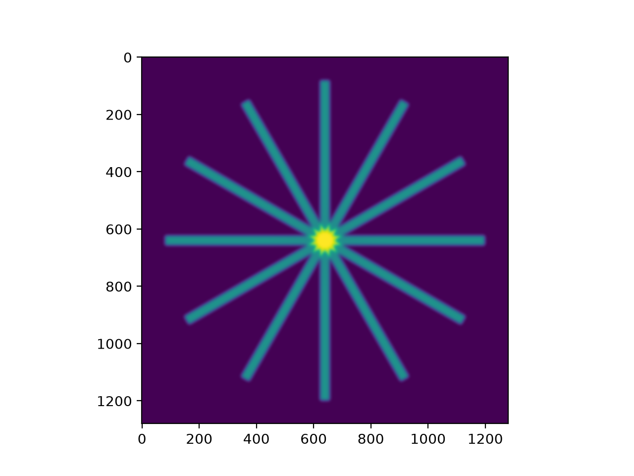
The basics to get started are to import the image simulators and layers from pylinac and add the layers as desired.
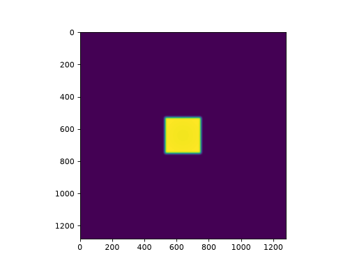
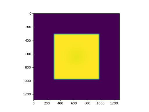
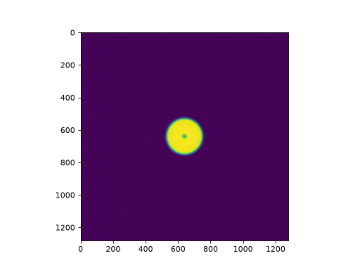
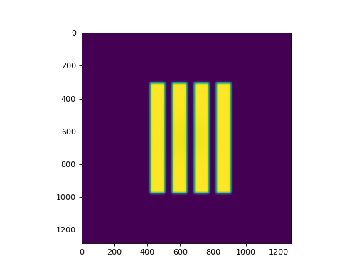
from matplotlib import pyplot as plt

from pylinac.core.image_generator import AS1200Image
from pylinac.core.image_generator.layers import FilteredFieldLayer, GaussianFilterLayer

as1200 = AS1200Image()  # this will set the pixel size and shape automatically
as1200.add_layer(FilteredFieldLayer(field_size_mm=(50, 50)))  # create a 50x50mm square field
as1200.add_layer(GaussianFilterLayer(sigma_mm=2))  # add an image-wide gaussian to simulate penumbra/scatter
as1200.generate_dicom(file_out_name="my_AS1200.dcm", gantry_angle=45)  # create a DICOM file with the simulated image
# plot the generated image
plt.imshow(as1200.image)
(Source code, png, hires.png, pdf)
Layers & Simulators
Layers are very simple structures. They usually have constructor arguments specific to the layer and always define an
apply method with the signature .apply(image, pixel_size) -> image. The apply method returns the modified image
(a numpy array). That’s it!
Simulators are also simple and define the parameters of the image to which layers are added. They have pixel_size
and shape properties and always have an add_layer method with the signature .add_layer(layer: Layer). They
also have a generate_dicom method for dumping the image along with mostly stock metadata to DICOM.
Extending Layers & Simulators
This module is meant to be extensible. That’s why the structures are defined so simply. To create a custom simulator,
inherit from Simulator and define the pixel size and shape:
from pylinac.core.image_generator.simulators import Simulator


class AS5000(Simulator):
    pixel_size = 0.12
    shape = (5000, 5000)


# use like any other simulator
To implement a custom layer, inherit from Layer and implement the apply method:
from pylinac.core.image_generator.layers import Layer


class MyAwesomeLayer(Layer):
    def apply(image, pixel_size):
        # do stuff here
        return image


# use
from pylinac.core.image_generator import AS1200Image

as1200 = AS1200Image()
as1200.add_layer(MyAwesomeLayer())
...
Exporting Images to DICOM
The Simulator class has two methods for generating DICOM. One returns a Dataset and another fully saves it out to a file.
from pylinac.core.image_generator import AS1200Image
from pylinac.core.image_generator.layers import FilteredFieldLayer, GaussianFilterLayer

as1200 = AS1200Image()
as1200.add_layer(FilteredFieldLayer(field_size_mm=(50, 50)))
as1200.add_layer(GaussianFilterLayer(sigma_mm=2))

# generate a pydicom Dataset
ds = as1200.as_dicom(gantry_angle=45)
# do something with that dataset as needed
ds.PatientID = "12345"

# or save it out to a file
as1200.generate_dicom(file_out_name="my_AS1200.dcm", gantry_angle=45)
Examples
Let’s make some images!
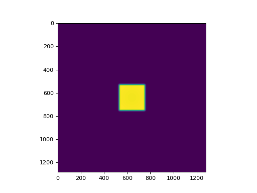
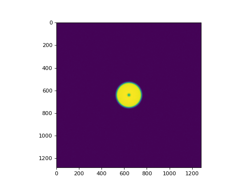
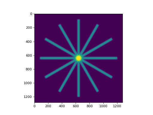
Simple Open Field
from matplotlib import pyplot as plt
from pylinac.core.image_generator import AS1200Image
from pylinac.core.image_generator.layers import FilteredFieldLayer, GaussianFilterLayer

as1200 = AS1200Image()  # this will set the pixel size and shape automatically
as1200.add_layer(FilteredFieldLayer(field_size_mm=(150, 150)))  # create a 50x50mm square field
as1200.add_layer(GaussianFilterLayer(sigma_mm=2))  # add an image-wide gaussian to simulate penumbra/scatter
# plot the generated image
plt.imshow(as1200.image)
(Source code, png, hires.png, pdf)
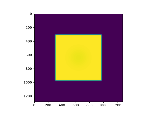
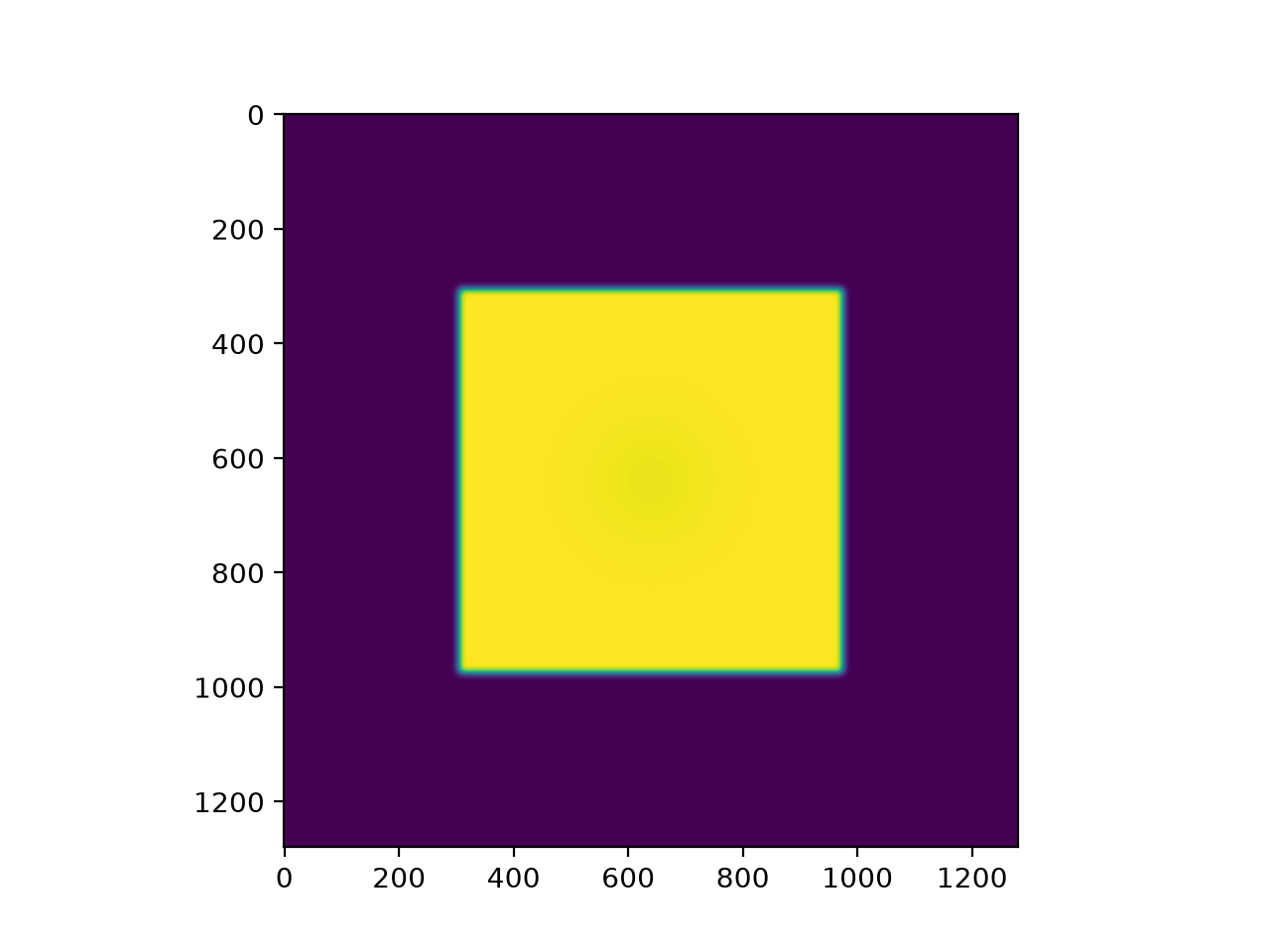
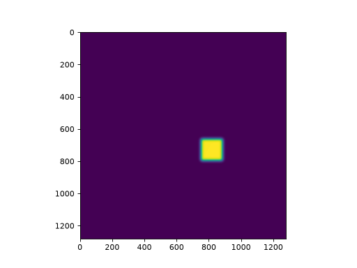
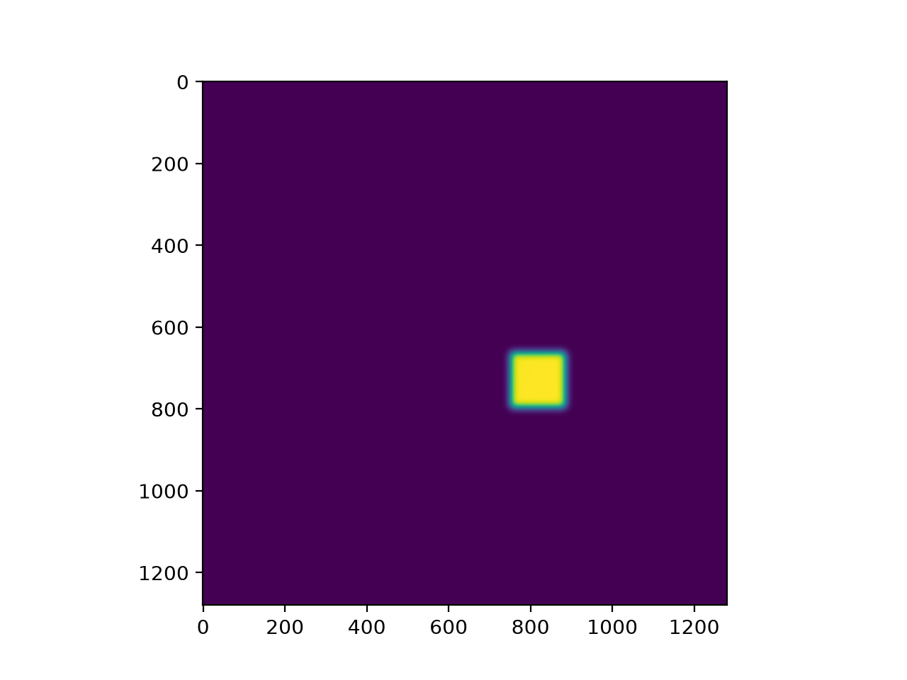
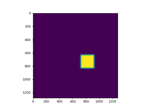
Off-center Open Field
from matplotlib import pyplot as plt
from pylinac.core.image_generator import AS1200Image
from pylinac.core.image_generator.layers import FilteredFieldLayer, GaussianFilterLayer

as1200 = AS1200Image()  # this will set the pixel size and shape automatically
as1200.add_layer(FilteredFieldLayer(field_size_mm=(30, 30), cax_offset_mm=(20, 40)))
as1200.add_layer(GaussianFilterLayer(sigma_mm=3))
# plot the generated image
plt.imshow(as1200.image)
(Source code, png, hires.png, pdf)
Winston-Lutz FFF Cone Field with Noise
from matplotlib import pyplot as plt
from pylinac.core.image_generator import AS1200Image
from pylinac.core.image_generator.layers import FilterFreeConeLayer, GaussianFilterLayer, PerfectBBLayer, RandomNoiseLayer

as1200 = AS1200Image()
as1200.add_layer(FilterFreeConeLayer(50))
as1200.add_layer(PerfectBBLayer(bb_size_mm=5))
as1200.add_layer(GaussianFilterLayer(sigma_mm=2))
as1200.add_layer(RandomNoiseLayer(sigma=0.02))
# plot the generated image
plt.imshow(as1200.image)
(Source code, png, hires.png, pdf)
VMAT DRMLC
from matplotlib import pyplot as plt
from pylinac.core.image_generator import AS1200Image
from pylinac.core.image_generator.layers import FilteredFieldLayer, GaussianFilterLayer

as1200 = AS1200Image()
as1200.add_layer(FilteredFieldLayer((150, 20), cax_offset_mm=(0, -40)))
as1200.add_layer(FilteredFieldLayer((150, 20), cax_offset_mm=(0, -10)))
as1200.add_layer(FilteredFieldLayer((150, 20), cax_offset_mm=(0, 20)))
as1200.add_layer(FilteredFieldLayer((150, 20), cax_offset_mm=(0, 50)))
as1200.add_layer(GaussianFilterLayer())
plt.imshow(as1200.image)
plt.show()
(Source code, png, hires.png, pdf)
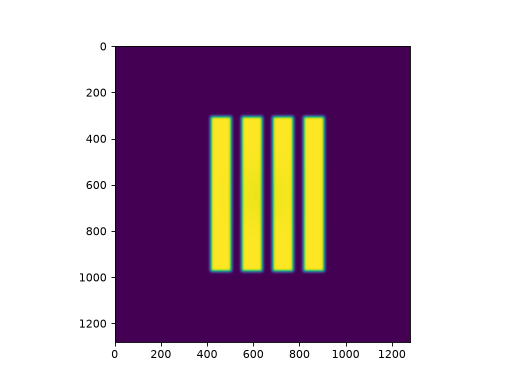
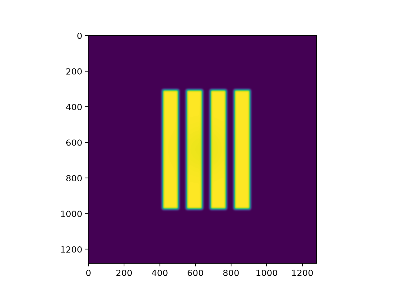
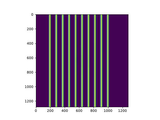
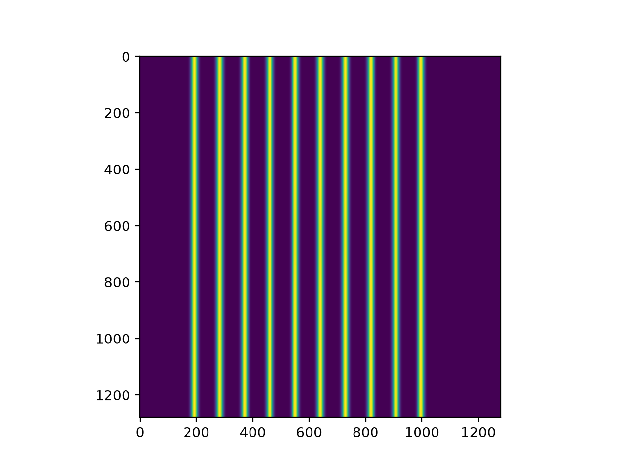
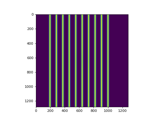
Picket Fence
from matplotlib import pyplot as plt
from pylinac.core.image_generator import AS1200Image
from pylinac.core.image_generator.layers import FilteredFieldLayer, GaussianFilterLayer

as1200 = AS1200Image()
height = 350
width = 4
offsets = range(-100, 100, 20)
for offset in offsets:
    as1200.add_layer(FilteredFieldLayer((height, width), cax_offset_mm=(0, offset)))
as1200.add_layer(GaussianFilterLayer())
plt.imshow(as1200.image)
plt.show()
(Source code, png, hires.png, pdf)
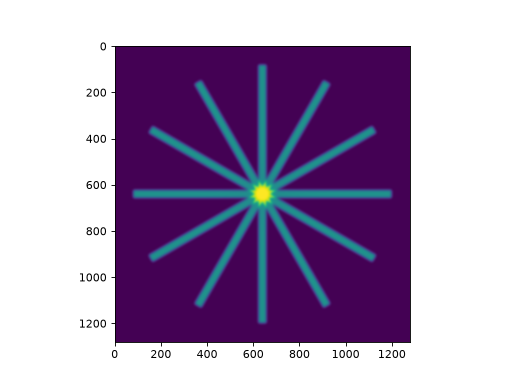
Starshot
Simulating a starshot requires a small trick as angled fields cannot be handled by default. The following example rotates the image after every layer is applied.
Note
Rotating the image like this is a convenient trick but note that it will rotate the entire existing image including all previous layers. This will also possibly erroneously adjust the horn effect simulation. Use with caution.
from scipy import ndimage
from matplotlib import pyplot as plt
from pylinac.core.image_generator import AS1200Image
from pylinac.core.image_generator.layers import FilteredFieldLayer, GaussianFilterLayer

as1200 = AS1200Image()
for _ in range(6):
    as1200.add_layer(FilteredFieldLayer((250, 7), alpha=0.5))
    as1200.image = ndimage.rotate(as1200.image, 30, reshape=False, mode='nearest')
as1200.add_layer(GaussianFilterLayer())
plt.imshow(as1200.image)
plt.show()
(Source code, png, hires.png, pdf)
Helper utilities
Using the new utility functions of v2.5+ we can construct full dicom files of picket fence and winston-lutz sets of images:
from pylinac.core.image_generator import generate_picketfence, generate_winstonlutz
from pylinac.core import image_generator

sim = image_generator.simulators.AS1200Image()
field_layer = image_generator.layers.FilteredFieldLayer  # could also do FilterFreeLayer
generate_picketfence(
    simulator=Simulator,
    field_layer=FilteredFieldLayer,
    file_out="pf_image.dcm",
    pickets=11,
    picket_spacing_mm=20,
    picket_width_mm=2,
    picket_height_mm=300,
    gantry_angle=0,
)
# we now have a pf image saved as 'pf_image.dcm'

# create a set of WL images
# this will create 4 images (via image_axes len) with an offset of 3mm to the left
# the function is smart enough to correct for the offset w/r/t gantry angle.
generate_winstonlutz(
    simulator=sim,
    field_layer=field_layer,
    final_layers=[GaussianFilterLayer()],
    gantry_tilt=0,
    dir_out="./wl_dir",
    offset_mm_left=3,
    image_axes=[[0, 0, 0], [180, 0, 0], [90, 0, 0], [270, 0, 0]],
)
Tips & Tricks
The
FilteredFieldLayerandFilterFree<Field, Cone>Layerhave gaussian filters applied to create a first-order approximation of the horn(s) of the beam. It doesn’t claim to be super-accurate, it’s just to give some reality to the images. You can adjust the magnitude of these parameters to simulate other energies (e.g. sharper horns) when defining the layer.The
Perfect...Layers do not apply any energy correction as above.Use
alphato adjust the intensity of the layer. E.g. the BB layer has a default alpha of -0.5 to simulate attenuation. This will subtract out up to half of the possible dose range existing on the image thus far (e.g. an open image of alpha 1.0 will be reduced to 0.5 after a BB is layered with alpha=-0.5). If you want to simulate a thick material like tungsten you can adjust the alpha to be lower (more attenuation). An alpha of 1 means full radiation, no attenuation (like an open field).Generally speaking, don’t apply more than one
GaussianFilterLayersince they are additive. A good rule is to apply one filter at the end of your layering.Apply
ConstantLayers at the beginning rather than the end.
Warning
Pylinac uses unsigned int16 datatypes (native EPID dtype). To keep images from flipping bits when adding layers,
pylinac will clip the values. Just be careful when, e.g. adding a ConstantLayer at the end of a layering. Better to do this
at the beginning.
API Documentation
Layers
- class pylinac.core.image_generator.layers.PerfectConeLayer(cone_size_mm: float = 10, cax_offset_mm: float, float = (0, 0), alpha: float = 1.0, rotation: float = 0)[source]
Bases:
LayerA cone without flattening filter effects
Parameters
- cone_size_mm
Cone size in mm at the iso plane
- cax_offset_mm
The offset in mm. (down, right)
- alpha
The intensity of the layer. 1 is full saturation/radiation. 0 is none.
- rotation: float
The amount of rotation in degrees. When there is an offset, this acts like a couch kick.
- apply(image: ndarray, pixel_size: float, mag_factor: float) ndarray[source]
Apply the layer. Takes a 2D array and pixel size value in and returns a modified array.
Parameters
- imagenp.ndarray
The image to modify.
- pixel_sizefloat
The pixel size of the image AT SAD.
- mag_factorfloat
The magnification factor of the image. SID/SAD. E.g. 1.5 for 150 cm SID and 100 cm SAD.
- class pylinac.core.image_generator.layers.FilterFreeConeLayer(cone_size_mm: float = 10, cax_offset_mm: float, float = (0, 0), alpha: float = 1.0, filter_magnitude: float = 0.4, filter_sigma_mm: float = 80)[source]
Bases:
PerfectConeLayerA cone with flattening filter effects.
Parameters
- cone_size_mm
Cone size in mm at the iso plane
- cax_offset_mm
The offset in mm. (out, right)
- alpha
The intensity of the layer. 1 is full saturation/radiation. 0 is none.
- filter_magnitude
The magnitude of the CAX peak. Larger values result in “pointier” fields.
- filter_sigma_mm
Proportional to the width of the CAX peak. Larger values produce wider curves.
- apply(image: ndarray, pixel_size: float, mag_factor: float) ndarray[source]
Apply the layer. Takes a 2D array and pixel size value in and returns a modified array.
Parameters
- imagenp.ndarray
The image to modify.
- pixel_sizefloat
The pixel size of the image AT SAD.
- mag_factorfloat
The magnification factor of the image. SID/SAD. E.g. 1.5 for 150 cm SID and 100 cm SAD.
- class pylinac.core.image_generator.layers.PerfectFieldLayer(field_size_mm: float, float = (10, 10), cax_offset_mm: float, float = (0, 0), alpha: float = 1.0, rotation: float = 0)[source]
Bases:
LayerA square field without flattening filter effects
Parameters
- field_size_mm
Field size in mm at the iso plane as (height, width)
- cax_offset_mm
The offset in mm. (down, right)
- alpha
The intensity of the layer. 1 is full saturation/radiation. 0 is none.
- rotation: float
The amount of rotation in degrees. This acts like a collimator rotation.
- apply(image: ndarray, pixel_size: float, mag_factor: float) array[source]
Apply the layer. Takes a 2D array and pixel size value in and returns a modified array.
Parameters
- imagenp.ndarray
The image to modify.
- pixel_sizefloat
The pixel size of the image AT SAD.
- mag_factorfloat
The magnification factor of the image. SID/SAD. E.g. 1.5 for 150 cm SID and 100 cm SAD.
- class pylinac.core.image_generator.layers.FilteredFieldLayer(field_size_mm: float, float = (10, 10), cax_offset_mm: float, float = (0, 0), alpha: float = 1.0, gaussian_height: float = 0.03, gaussian_sigma_mm: float = 32, rotation: float = 0)[source]
Bases:
PerfectFieldLayerA square field with flattening filter effects
Parameters
- field_size_mm
Field size in mm at the iso plane (height, width)
- cax_offset_mm
The offset in mm. (out, right)
- alpha
The intensity of the layer. 1 is full saturation/radiation. 0 is none.
- gaussian_height
The intensity of the “horns”, or more accurately, the CAX dip. Proportional to the max value allowed for the data type. Increase to make the horns more prominent.
- gaussian_sigma_mm
The width of the “horns”. A.k.a. the CAX dip width. Increase to create a wider horn effect.
- rotation: float
The amount of rotation in degrees. This acts like a collimator rotation.
- apply(image: array, pixel_size: float, mag_factor: float) array[source]
Apply the layer. Takes a 2D array and pixel size value in and returns a modified array.
Parameters
- imagenp.ndarray
The image to modify.
- pixel_sizefloat
The pixel size of the image AT SAD.
- mag_factorfloat
The magnification factor of the image. SID/SAD. E.g. 1.5 for 150 cm SID and 100 cm SAD.
- class pylinac.core.image_generator.layers.FilterFreeFieldLayer(field_size_mm: float, float = (10, 10), cax_offset_mm: float, float = (0, 0), alpha: float = 1.0, gaussian_height: float = 0.4, gaussian_sigma_mm: float = 80, rotation: float = 0)[source]
Bases:
FilteredFieldLayerA square field with flattening filter free (FFF) effects
Parameters
- field_size_mm
Field size in mm at the iso plane (height, width).
- cax_offset_mm
The offset in mm. (out, right)
- alpha
The intensity of the layer. 1 is full saturation/radiation. 0 is none.
- gaussian_height
The magnitude of the CAX peak. Larger values result in “pointier” fields.
- gaussian_sigma_mm
Proportional to the width of the CAX peak. Larger values produce wider curves.
- rotation: float
The amount of rotation in degrees. This acts like a collimator rotation.
- apply(image: array, pixel_size: float, mag_factor: float) array[source]
Apply the layer. Takes a 2D array and pixel size value in and returns a modified array.
Parameters
- imagenp.ndarray
The image to modify.
- pixel_sizefloat
The pixel size of the image AT SAD.
- mag_factorfloat
The magnification factor of the image. SID/SAD. E.g. 1.5 for 150 cm SID and 100 cm SAD.
- class pylinac.core.image_generator.layers.PerfectBBLayer(bb_size_mm: float = 5, cax_offset_mm: float, float = (0, 0), alpha: float = -0.5, rotation: float = 0)[source]
Bases:
PerfectConeLayerA BB-like layer. Like a cone, but with lower alpha (i.e. higher opacity)
Parameters
- cone_size_mm
Cone size in mm at the iso plane
- cax_offset_mm
The offset in mm. (down, right)
- alpha
The intensity of the layer. 1 is full saturation/radiation. 0 is none.
- rotation: float
The amount of rotation in degrees. When there is an offset, this acts like a couch kick.
- apply(image: ndarray, pixel_size: float, mag_factor: float) ndarray
Apply the layer. Takes a 2D array and pixel size value in and returns a modified array.
Parameters
- imagenp.ndarray
The image to modify.
- pixel_sizefloat
The pixel size of the image AT SAD.
- mag_factorfloat
The magnification factor of the image. SID/SAD. E.g. 1.5 for 150 cm SID and 100 cm SAD.
- class pylinac.core.image_generator.layers.GaussianFilterLayer(sigma_mm: float = 2)[source]
Bases:
LayerA Gaussian filter. Simulates the effects of scatter on the field
- apply(image: array, pixel_size: float, mag_factor: float) array[source]
Apply the layer. Takes a 2D array and pixel size value in and returns a modified array.
Parameters
- imagenp.ndarray
The image to modify.
- pixel_sizefloat
The pixel size of the image AT SAD.
- mag_factorfloat
The magnification factor of the image. SID/SAD. E.g. 1.5 for 150 cm SID and 100 cm SAD.
- class pylinac.core.image_generator.layers.RandomNoiseLayer(mean: float = 0.0, sigma: float = 0.001)[source]
Bases:
LayerA salt and pepper noise, simulating dark current
- apply(image: array, pixel_size: float, mag_factor: float) array[source]
Apply the layer. Takes a 2D array and pixel size value in and returns a modified array.
Parameters
- imagenp.ndarray
The image to modify.
- pixel_sizefloat
The pixel size of the image AT SAD.
- mag_factorfloat
The magnification factor of the image. SID/SAD. E.g. 1.5 for 150 cm SID and 100 cm SAD.
- class pylinac.core.image_generator.layers.ConstantLayer(constant: float)[source]
Bases:
LayerA constant layer. Can be used to simulate scatter or background.
- apply(image: array, pixel_size: float, mag_factor: float) array[source]
Apply the layer. Takes a 2D array and pixel size value in and returns a modified array.
Parameters
- imagenp.ndarray
The image to modify.
- pixel_sizefloat
The pixel size of the image AT SAD.
- mag_factorfloat
The magnification factor of the image. SID/SAD. E.g. 1.5 for 150 cm SID and 100 cm SAD.
- class pylinac.core.image_generator.layers.SlopeLayer(slope_x: float, slope_y: float)[source]
Bases:
LayerAdds a slope in both directions of the image. Usually used for simulating asymmetry or a-flatness.
Parameters
- slope_xfloat
The slope in the x-direction (left/right). If positive, will increase the right side. The value is multiplicative to the current state of the image. E.g. a value of 0.1 will increase the right side by 10% and 0% on the left.
- slope_yfloat
The slope in the y-direction (up/down). If positive, will increase the bottom side.
- apply(image: ndarray, pixel_size: float, mag_factor: float) ndarray[source]
Apply the layer. Takes a 2D array and pixel size value in and returns a modified array.
Parameters
- imagenp.ndarray
The image to modify.
- pixel_sizefloat
The pixel size of the image AT SAD.
- mag_factorfloat
The magnification factor of the image. SID/SAD. E.g. 1.5 for 150 cm SID and 100 cm SAD.
- class pylinac.core.image_generator.layers.ArrayLayer(image: ndarray)[source]
Bases:
LayerAdd an already-existing array as a layer. Useful if the array is already constructed to your liking. Simply passes the array given. It is the caller’s responsibility to know the array to pass and that the pixel size has been accounted for already.
If the passed array is smaller than the simulator’s image, it will be centered on the simulator image and added. If the passed array is bigger than the simulator’s image, it will be centered, cropped to fit the simulator’s array size, and then added.
Parameters
- imagenp.ndarray
The array to add to the simulator image.
- apply(image: ndarray, pixel_size: float, mag_factor: float) ndarray[source]
Apply the layer. Takes a 2D array and pixel size value in and returns a modified array.
Parameters
- imagenp.ndarray
The image to modify.
- pixel_sizefloat
The pixel size of the image AT SAD.
- mag_factorfloat
The magnification factor of the image. SID/SAD. E.g. 1.5 for 150 cm SID and 100 cm SAD.
Simulators
- class pylinac.core.image_generator.simulators.AS500Image(sid: float = 1500)[source]
Bases:
SimulatorSimulates an AS500 EPID image.
Parameters
- sid
Source to image distance in mm.
- add_layer(layer: Layer) None
Add a layer to the image
- as_dicom(gantry_angle: float = 0.0, coll_angle: float = 0.0, table_angle: float = 0.0, invert_array: bool = False, tags: dict | None = None) Dataset
Create and return a pydicom Dataset. I.e. create a pseudo-DICOM image.
- generate_dicom(file_out_name: str, *args, **kwargs) None
Save the simulated image to a DICOM file.
See Also
as_dicom
- plot(show: bool = True) Figure
Plot the simulated image.
- class pylinac.core.image_generator.simulators.AS1000Image(sid: float = 1500)[source]
Bases:
SimulatorSimulates an AS1000 EPID image.
Parameters
- sid
Source to image distance in mm.
- add_layer(layer: Layer) None
Add a layer to the image
- as_dicom(gantry_angle: float = 0.0, coll_angle: float = 0.0, table_angle: float = 0.0, invert_array: bool = False, tags: dict | None = None) Dataset
Create and return a pydicom Dataset. I.e. create a pseudo-DICOM image.
- generate_dicom(file_out_name: str, *args, **kwargs) None
Save the simulated image to a DICOM file.
See Also
as_dicom
- plot(show: bool = True) Figure
Plot the simulated image.
- class pylinac.core.image_generator.simulators.AS1200Image(sid: float = 1500)[source]
Bases:
SimulatorSimulates an AS1200 EPID image.
Parameters
- sid
Source to image distance in mm.
- add_layer(layer: Layer) None
Add a layer to the image
- as_dicom(gantry_angle: float = 0.0, coll_angle: float = 0.0, table_angle: float = 0.0, invert_array: bool = False, tags: dict | None = None) Dataset
Create and return a pydicom Dataset. I.e. create a pseudo-DICOM image.
- generate_dicom(file_out_name: str, *args, **kwargs) None
Save the simulated image to a DICOM file.
See Also
as_dicom
- plot(show: bool = True) Figure
Plot the simulated image.
Helpers
- pylinac.core.image_generator.utils.generate_picketfence(simulator: Simulator, field_layer: type[FilterFreeFieldLayer | FilteredFieldLayer | PerfectFieldLayer], file_out: str, final_layers: list[Layer] = None, pickets: int = 11, picket_spacing_mm: float = 20, picket_width_mm: int = 2, picket_height_mm: int = 300, gantry_angle: int = 0, orientation: Orientation = Orientation.UP_DOWN, picket_offset_error: Sequence | None = None) None[source]
Create a mock picket fence image. Will always be up-down.
Parameters
- simulator
The image simulator
- field_layer
The primary field layer
- file_out
The name of the file to save the DICOM file to.
- final_layers
Optional layers to apply at the end of the procedure. Useful for noise or blurring.
- pickets
The number of pickets
- picket_spacing_mm
The space between pickets
- picket_width_mm
Picket width parallel to leaf motion
- picket_height_mm
Picket height parallel to leaf motion
- gantry_angle
Gantry angle; sets the DICOM tag.
- pylinac.core.image_generator.utils.generate_winstonlutz(simulator: Simulator, field_layer: type[Layer], dir_out: str, field_size_mm: tuple[float, float] = (30, 30), final_layers: list[Layer] | None = None, bb_size_mm: float = 5, offset_mm_left: float = 0, offset_mm_up: float = 0, offset_mm_in: float = 0, image_axes: int, int, int, ... = ((0, 0, 0), (90, 0, 0), (180, 0, 0), (270, 0, 0)), machine_scale: MachineScale = MachineScale.IEC61217, gantry_tilt: float = 0, gantry_sag: float = 0, clean_dir: bool = True, field_alpha: float = 1.0, bb_alpha: float = -0.5, tags: dict | None = None) list[str][source]
Create a mock set of WL images. Used for benchmarking the WL algorithm. Produces one image for each item in
image_axes.Parameters
- simulator
The image simulator
- field_layer
The primary field layer simulating radiation
- dir_out
The directory to save the images to.
- field_size_mm
The field size of the radiation field in mm
- final_layers
Layers to apply after generating the primary field and BB layer. Useful for blurring or adding noise.
- bb_size_mm
The size of the BB. Must be positive.
- offset_mm_left
How far left (LAT) to set the BB. Can be positive or negative.
- offset_mm_up
How far up (VERT) to set the BB. Can be positive or negative.
- offset_mm_in
How far in (LONG) to set the BB. Can be positive or negative.
- image_axes
List of axis values for the images. Sequence is (Gantry, Coll, Couch).
- machine_scale
The scale of the machine. Will convert to IEC61217. Allows users to enter image_axes in their machine’s scale if desired.
- gantry_tilt
The tilt of the gantry that affects the position at 0 and 180. Simulates a simple cosine function.
- gantry_sag
The sag of the gantry that affects the position at gantry=90 and 270. Simulates a simple sine function.
- clean_dir
Whether to clean out the output directory. Useful when iterating.
- field_alpha
The normalized alpha (i.e. signal) of the radiation field. Use in combination with bb_alpha such that the sum of the two is always <= 1.
- bb_alpha
The normalized alpha (in the case of the BB think of it as attenuation) of the BB against the radiation field. More negative values attenuate (remove signal) more.
- tags
Extra DICOM tags that will be applied to all the DICOM files generated.
- pylinac.core.image_generator.utils.generate_winstonlutz_cone(simulator: Simulator, cone_layer: type[FilterFreeConeLayer] | type[PerfectConeLayer], dir_out: str, cone_size_mm: float = 17.5, final_layers: list[Layer] | None = None, bb_size_mm: float = 5, offset_mm_left: float = 0, offset_mm_up: float = 0, offset_mm_in: float = 0, image_axes: int, int, int, ... = ((0, 0, 0), (90, 0, 0), (180, 0, 0), (270, 0, 0)), gantry_tilt: float = 0, gantry_sag: float = 0, clean_dir: bool = True) list[str][source]
Create a mock set of WL images with a cone field, simulating gantry sag effects. Produces one image for each item in image_axes.
Parameters
- simulator
The image simulator
- cone_layer
The primary field layer simulating radiation
- dir_out
The directory to save the images to.
- cone_size_mm
The field size of the radiation field in mm
- final_layers
Layers to apply after generating the primary field and BB layer. Useful for blurring or adding noise.
- bb_size_mm
The size of the BB. Must be positive.
- offset_mm_left
How far left (lat) to set the BB. Can be positive or negative.
- offset_mm_up
How far up (vert) to set the BB. Can be positive or negative.
- offset_mm_in
How far in (long) to set the BB. Can be positive or negative.
- image_axes
List of axis values for the images. Sequence is (Gantry, Coll, Couch).
- gantry_tilt
The tilt of the gantry in degrees that affects the position at 0 and 180. Simulates a simple cosine function.
- gantry_sag
The sag of the gantry that affects the position at gantry=90 and 270. Simulates a simple sine function.
- clean_dir
Whether to clean out the output directory. Useful when iterating.
- pylinac.core.image_generator.utils.generate_winstonlutz_multi_bb_multi_field(simulator: Simulator, field_layer: type[Layer], dir_out: str, field_offsets: Sequence[Sequence[float]], bb_offsets: Sequence[Sequence[float]] | list[dict[str, float]], field_size_mm: tuple[float, float] = (20, 20), final_layers: Sequence[Layer] | None = None, bb_size_mm: float = 5, image_axes: int, int, int, ... = ((0, 0, 0), (90, 0, 0), (180, 0, 0), (270, 0, 0)), gantry_tilt: float = 0, gantry_sag: float = 0, clean_dir: bool = True, jitter_mm: float = 0, align_to_pixels: bool = True) list[str][source]
Create a mock set of WL images, simulating gantry sag effects. Produces one image for each item in image_axes. This will also generate multiple BBs on the image, one per item in offsets. Each offset should be a list of the shifts of the BB relative to isocenter like so: [<left>, <up>, <in>] OR an arrangement from the WL module.
Parameters
- simulator
The image simulator
- field_layer
The primary field layer simulating radiation
- dir_out
The directory to save the images to.
- field_offsets
A list of lists containing the shift of the fields. Format is the same as bb_offsets.
- bb_offsets
A list of lists containing the shift of the BBs from iso; each sublist should be a 3-item list/tuple of left, up, in. Negative values are acceptable and will go the opposite direction.
- field_size_mm
The field size of the radiation field in mm
- final_layers
Layers to apply after generating the primary field and BB layer. Useful for blurring or adding noise.
- bb_size_mm
The size of the BB. Must be positive.
- image_axes
List of axis values for the images. Sequence is (Gantry, Coll, Couch).
- gantry_tilt
The tilt of the gantry in degrees that affects the position at 0 and 180. Simulates a simple cosine function.
- gantry_sag
The sag of the gantry that affects the position at gantry=90 and 270. Simulates a simple sine function.
- clean_dir
Whether to clean out the output directory. Useful when iterating.
- jitter_mm
The amount of jitter to add to the in/left/up location of the BB in MM.