Log Analyzer
Overview
The log analyzer module reads and parses Varian linear accelerator machine logs, both Dynalogs and Trajectory logs. The module also calculates actual and expected fluences as well as performing gamma evaluations. Data is structured to be easily accessible and easily plottable.
Unlike most other modules of pylinac, the log analyzer module has no end goal. Data is parsed from the logs, but what is done with that info, and which info is analyzed is up to the user.
Features:
Analyze Dynalogs or Trajectory logs - Either platform is supported. Tlog versions 2.1, 3.0, and 4.0 are supported.
Read in both .bin and .txt Trajectory log files - Read in the machine data from both .bin and .txt files to get all the information recorded. See the
txtattribute.Save Trajectory log data to CSV - The Trajectory log binary data format does not allow for easy export of data. Pylinac lets you do that so you can use Excel or other software that you use with Dynalogs.
Plot or analyze any axis - Every data axis (e.g. gantry, y1, beam holds, MLC leaves) can be accessed and plotted: the actual, expected, and even the difference.
Calculate fluences and gamma - Besides reading in the MLC positions, pylinac calculates the actual and expected fluence as well as the gamma map; DTA and threshold values are adjustable.
Anonymize logs - Both dynalogs and trajectory logs can be “anonymized” by removing the Patient ID from the filename(s) and file data.
Concepts
Because the log_analyzer module functions without an end goal, the data has been formatted for easy exploration. However, there are a
few concepts that should be grasped before diving in.
Log Sections - Upon log parsing, all data is placed into data structures. Varian has designated 4 sections for Trajectory logs: Header, Axis Data, Subbeams, and CRC. The Subbeams are only applicable for auto-sequenced beams and all v3.0 logs, and the CRC is specific to the Trajectory log. The Header and Axis Data however, are common to both Trajectory logs and Dynalogs.
Note
Dynalogs do not have explicit sections like the Trajectory logs, but pylinac formats them to have these two data structures for consistency.
Leaf Indexing & Positions - Varian leaf identification is 1-index based, over against Python’s 0-based indexing. Thus, indexing the first MLC leaf would be
[1], not[0].Warning
When slicing or analyzing leaf data, keep the Varian 1-index base in mind.
Leaf data is stored in a dictionary, with the leaf number as the key, from 1 up to the number of MLC leaves. E.g. if the machine has a Millennium 120 standard MLC model, leaf data will have 120 dictionary items from 1 to 120. Leaves from each bank have an offset of half the number of leaves. I.e. leaves A1 and B1 = 1 and 61. Thus, leaves 61-120 correspond to the B-bank, while leaves 1-60 correspond to the A-bank. This can be described by a function \((A_{n}, B_{n}) = (n, n + N_{leaves}/2)\), where \(n\) is the leaf number and \(N_{leaves}\) is the number of leaves.
Units - Units follow the Trajectory log specification: linear axes are in cm, rotational axes in degrees, and MU for dose.
Note
Dynalog files are inherently in mm for collimator and gantry axes, tenths of degrees for rotational axes, and MLC positions are not at isoplane. For consistency, Dynalog values are converted to Trajectory log specs, meaning linear axes, both collimator and MLCs are in cm at isoplane, and rotational axes are in degrees. Dynalog MU is always from 0 to 25000 no matter the delivered MU (i.e. it’s relative), unless it was a VMAT delivery, in which case the gantry position is substituted in the dose fraction column.
Warning
Dynalog VMAT files replace the dose fraction column with the gantry position. Unfortunately, because of the variable dose rate of Varian linacs the gantry position is not a perfect surrogate for dose, but there is no other choice. Thus, fluence calculations will use the relative gantry movement as the dose in fluence calculations.
All data Axes are similar - Log files capture machine data in “control cycles”, aka “snapshots” or “heartbeats”. Let’s assume a log has captured 100 control cycles. Axis data that was captured will all be similar (e.g. gantry, collimator, jaws). They will all have an actual and sometimes an expected value for each cycle. Pylinac formats these as 1D numpy arrays along with a difference array if applicable. Each of these arrays can be quickly plotted for visual analysis. See
Axisfor more info.
Running the Demos
As usual, the module comes with demo files and methods:
from pylinac import Dynalog

Dynalog.run_demo()
Which will output the following:
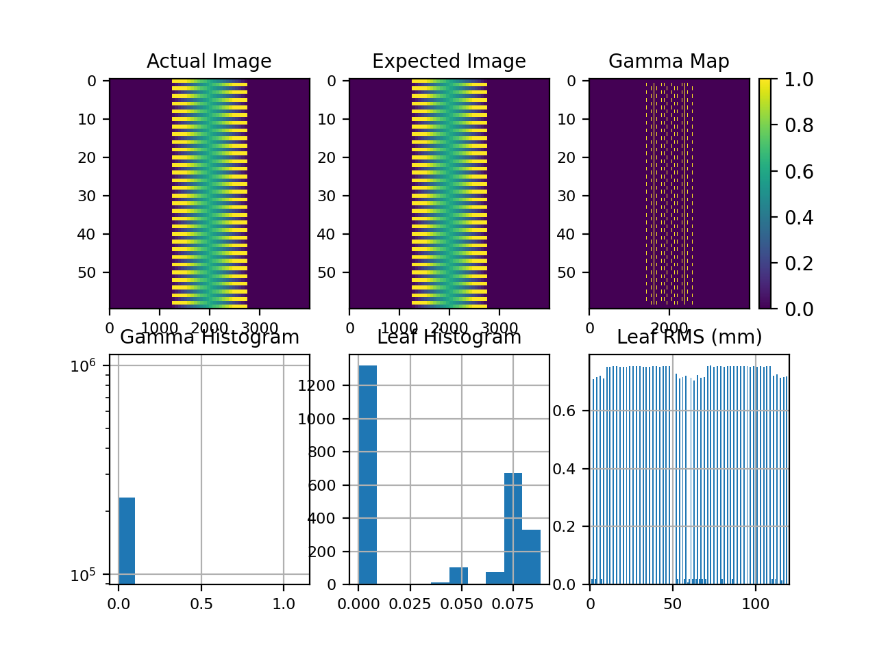
Results of file: C:\Users\James\Dropbox\Programming\Python\Projects\pylinac\pylinac\demo_files\AQA.dlg
Average RMS of all leaves: 0.037 cm
Max RMS error of all leaves: 0.076 cm
95th percentile error: 0.088 cm
Number of beam holdoffs: 20
Gamma pass %: 18.65
Gamma average: 0.468
(Source code, png, hires.png, pdf)

Your file location will be different, but the values should be the same. The same can be done using the demo Trajectory log:
from pylinac import TrajectoryLog

TrajectoryLog.run_demo()
Which will give:
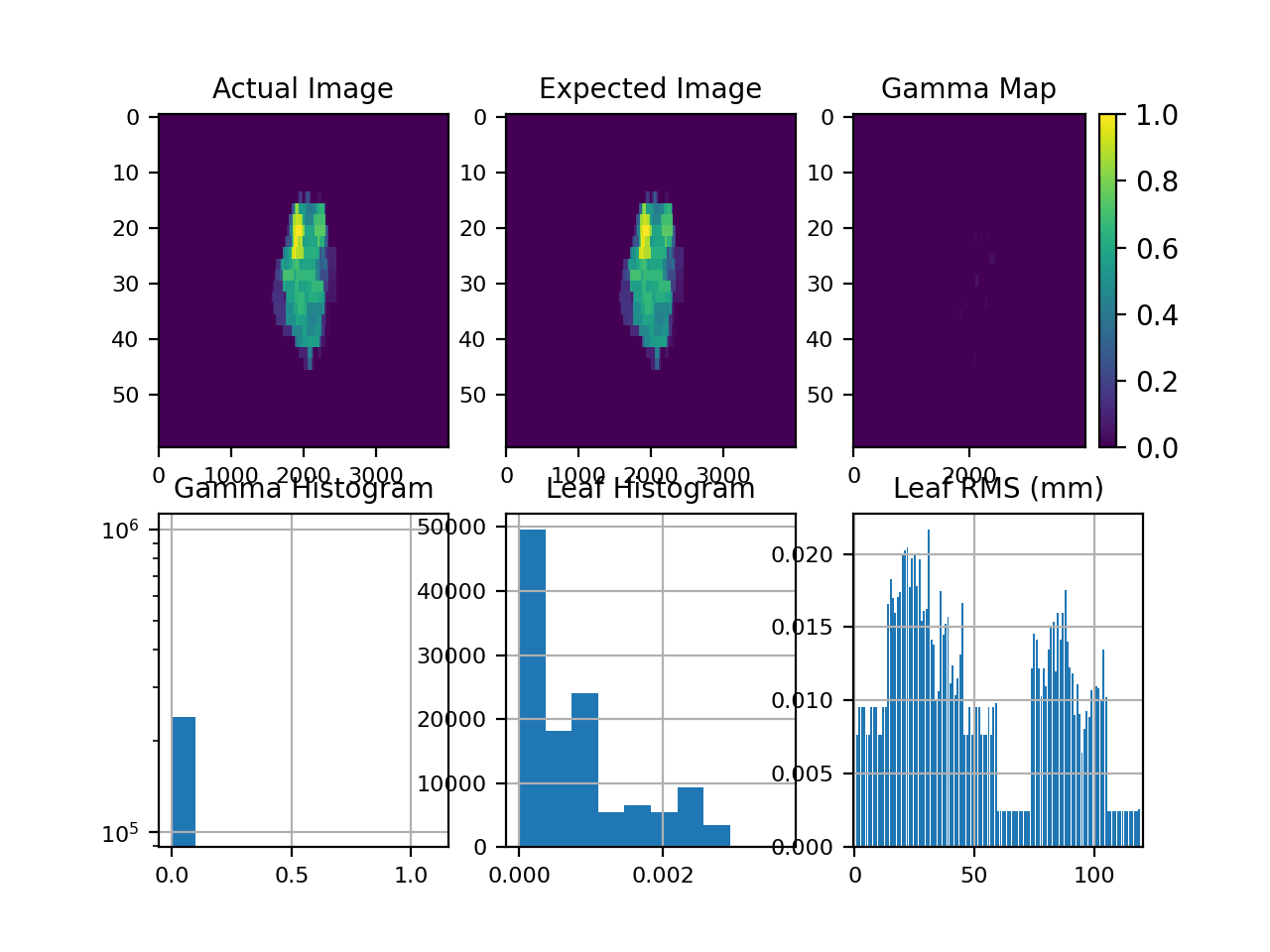
Results of file: C:\Users\James\Dropbox\Programming\Python\Projects\pylinac\pylinac\demo_files\Tlog.bin
Average RMS of all leaves: 0.001 cm
Max RMS error of all leaves: 0.002 cm
95th percentile error: 0.002 cm
Number of beam holdoffs: 19
Gamma pass %: 100.00
Gamma average: 0.002
(Source code, png, hires.png, pdf)

Note that you can also save data in a PDF report:
tlog = ...
tlog.publish_pdf("mytlog.pdf")
Loading Data
Loading Single Logs
Logs can be loaded two ways.
The first way is through the main helper function load_log().
Note
If you’ve used pylinac versions <1.6
the helper function is new and can be a replacement for MachineLog and MachineLogs, depending on the context
as discussed below.
from pylinac import load_log

log_path = "C:/path/to/tlog.bin"
log = load_log(log_path)
In addition, a folder, ZIP archive, or URL can also be passed:
log2 = load_log("http://myserver.com/logs/2.dlg")
Note
If loading from a URL the object can be a file or ZIP archive.
Pylinac will automatically infer the log type and load it into the appropriate data structures for analysis.
The load_log() function is a convenient wrapper around the classes within the log analysis module.
However, logs can be instantiated a second way: directly through the classes.
from pylinac import Dynalog, TrajectoryLog

dlog_path = "C:/path/to/dlog.dlg"
dlog = Dynalog(dlog_path)

tlog_path = "C:/path/to/tlog.bin"
tlog = TrajectoryLog(tlog_path)
Loading Multiple Logs
Loading multiple files is also possible using the load_log() function as listed above.
The logs can also be directly instantiated by using MachineLogs. Acceptable inputs include a folder and zip archive.
from pylinac import load_log, MachineLogs

path_to_folder = "C:/path/to/dir"

# from folder; equivalent
logs = MachineLogs(path_to_folder)
logs = load_log(path_to_folder)

# from ZIP archive
logs = load_log("path/to/logs.zip")
Working with the Data
Working with the log data is straightforward once the data structures and Axes are understood
(See Concepts for more info). Pylinac follows the data structures specified by Varian for
trajectory logs, with a Header and Axis Data structure, and possibly a Subbeams structure if
the log is a Trajectory log and was autosequenced. For accessible attributes, see TrajectoryLog. The
following sections explore each major section of log data and the data structures pylinac creates to assist
in data analysis.
Note
It may be helpful to also read the log specification format in parallel with this guide. It is easier to see that pylinac follows the log specifications and where the info comes from. Log specifications are on MyVarian.com.
Working with the Header
Header information is essentially anything that isn’t axis measurement data; it’s metadata about the file, format, machine configuration, etc. Because of the different file formats, there are separate classes for Trajectory log and Dynalog headers. The classes are:
Header attributes are listed in the class API docs by following the above links. For completeness they are also listed here. For Trajectory logs:
headerversionheader_sizesampling_intervalnum_axesaxis_enumsamples_per_axisnum_mlc_leavesaxis_scalenum_subbeamsis_truncatednum_snapshotsmlc_model
For Dynalogs the following header information is available:
versionpatient_nameplan_filenametolerancenum_mlc_leavesclinac_scale
Example
Let’s explore the header of the demo trajectory log:
>>> tlog = TrajectoryLog.from_demo()
>>> tlog.header.header
'VOSTL'
>>> tlog.header.version
2.1
>>> tlog.header.num_subbeams
2
Working with Axis Data
Axis data is all the information relating to the measurements of the various machine axes and is accessible
under the axis_data attribute. This includes the gantry,
collimator, MLCs, etc. Trajectory logs capture more information than Dynalogs, and additionally hold the expected
positions not only for MLCs but also for all axes. Every measurement axis has Axis as
its base; they all have similar methods to access and plot the data (see Plotting & Saving Axes/Fluences). However, not all attributes
are axes. Pylinac adds properties to the axis data structure for ease of use (e.g. the number of snapshots)
For Trajectory logs the following attributes are available,
based on the TrajectoryLogAxisData class:
collimatorgantryjawsNote
The
jawsattribute is a data structure to hold all 4 jaw axes; seeJawStructcouchNote
The
couchattribute is a data structure to hold lateral, longitudinal, etc couch positions; seeCouchStructmubeam_holdcontrol_pointcarriage_Acarriage_BmlcNote
The
mlcattribute is a data structure to hold leaf information; seeMLCfor attributes and the Working with MLC Data section for more info.
Dynalogs have similar attributes, derived from the DynalogAxisData class:
collimatorgantryjawsNote
The
jawsattribute is a data structure to hold all 4 jaw axes; seeJawStructnum_snapshotsmubeam_holdbeam_onprevious_segment_numprior_dose_indexnext_dose_indexcarriage_Acarriage_BmlcNote
The
mlcattribute is a data structure to hold leaf information; seeMLCfor attributes and the Working with MLC Data section for more info.
Example
Let’s access a few axis data attributes:
>>> log = Dynalog.from_demo()
>>> log.axis_data.mu.actual  # a numpy array
array([  0, 100, ...
>>> log.axis_data.num_snapshots
99
>>> log.axis_data.gantry.actual
array([ 180, 180, 180, ...
Working with MLC Data
Although MLC data is acquired and included in Trajectory logs and Dynalogs, it is not always easy to parse. Additionally,
a physicist may be interested in the MLC metrics of a log (RMS, etc). Pylinac provides tools for accessing MLC raw data as
well as helper methods and properties via the MLC class. Note that this class is consistent
between Trajectory logs and Dynalogs. This class is reachable through the axis_data
attribute as mlc.
Accessing Leaf data
Leaf data for any leaf is available under the leaf_axes attribute which is a dict. The leaves are keyed
by the leaf number and the value is an Axis. Example:
>>> log = Dynalog.from_demo()
>>> log.axis_data.mlc.leaf_axes[1].actual  # numpy array of the 'actual' values for leaf #1
array([ 7.56374, ...
>>> log.axis_data.mlc.leaf_axes[84].difference  # actual values minus the planned values for leaf 84
array([-0.001966, ...
MLC helper methods/properties
Beyond direct MLC data, pylinac provides a number of helper methods and properties to make working with MLC data easier
and more helpful. All the methods are listed in the MLC class, but some examples of use
are given here:
>>> log = Dynalog.from_demo()
>>> log.axis_data.mlc.get_error_percentile(percentile=95)  # get an MLC error percentile value
0.08847
>>> log.axis_data.mlc.leaf_moved(12)  # did leaf 12 move during treatment?
False
>>> log.axis_data.mlc.get_RMS_avg()  # get the average RMS error
0.03733
>>> log.axis_data.mlc.get_RMS_avg('A')  # get the average RMS error for bank A
0.03746
>>> log.axis_data.mlc.num_leaves  # the number of MLC leaves
120
>>> log.axis_data.mlc.num_moving_leaves  # the number of leaves that moved during treatment
60
Working with Fluences
Fluences created by the MLCs can also be accessed and viewed. Fluences are accessible under the fluence
attribute. There are three subclasses that handle the fluences:
The fluence actually delivered is in ActualFluence, the fluence planned is in
ExpectedFluence, and the gamma of the fluences is in GammaFluence.
Each fluence must be calculated, however pylinac makes reasonable defaults and has a few shortcuts. The actual and
expected fluences can be calculated to any resolution in the leaf-moving direction. Some examples:
>>> log = Dynalog.from_demo()
>>> log.fluence.actual.calc_map()  # calculate the actual fluence; returns a numpy array
array([ 0, 0, ...
>>> log.fluence.expected.calc_map(resolution=1)  # calculate at 1mm resolution
array([ 0, 0, ...
>>> log.fluence.gamma.calc_map(distTA=0.5, doseTA=1, resolution=0.1)  # change the gamma criteria
array([ 0, 0, ...
>>> log.fluence.gamma.pass_prcnt  # the gamma passing percentage
99.82
>>> log.fluence.gamma.avg_gamma  # the average gamma value
0.0208
Plotting & Saving Axes/Fluences
Each and every axis of the log can be accessed as a numpy array and/or plotted. For each axis the “actual” array/plot is always available. Dynalogs only have expected values for the MLCs. Trajectory logs have the actual and expected values for all axes. Additionally, if an axis has actual and expected arrays, then the difference is also available.
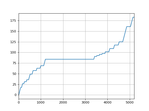
Example of plotting the MU actual:
import pylinac

log = pylinac.TrajectoryLog.from_demo()
log.axis_data.mu.plot_actual()
(Source code, png, hires.png, pdf)
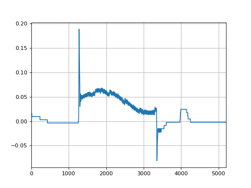
Plot the Gantry difference:
plt.clf()
log.axis_data.gantry.plot_difference()
(Source code, png, hires.png, pdf)

Axis plots are just as easily saved:
log.axis_data.gantry.save_plot_difference(filename="gantry diff.png")
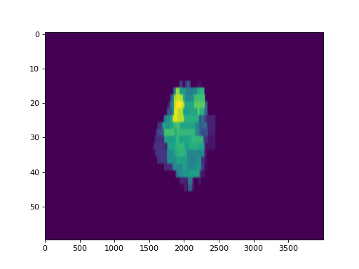
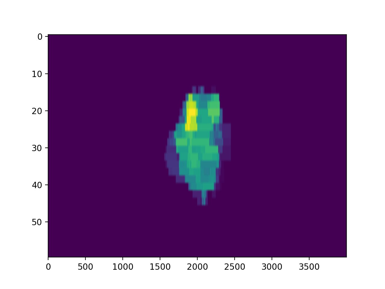
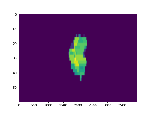
Now, lets plot the actual fluence:
log.fluence.actual.calc_map()
log.fluence.actual.plot_map()
(Source code, png, hires.png, pdf)

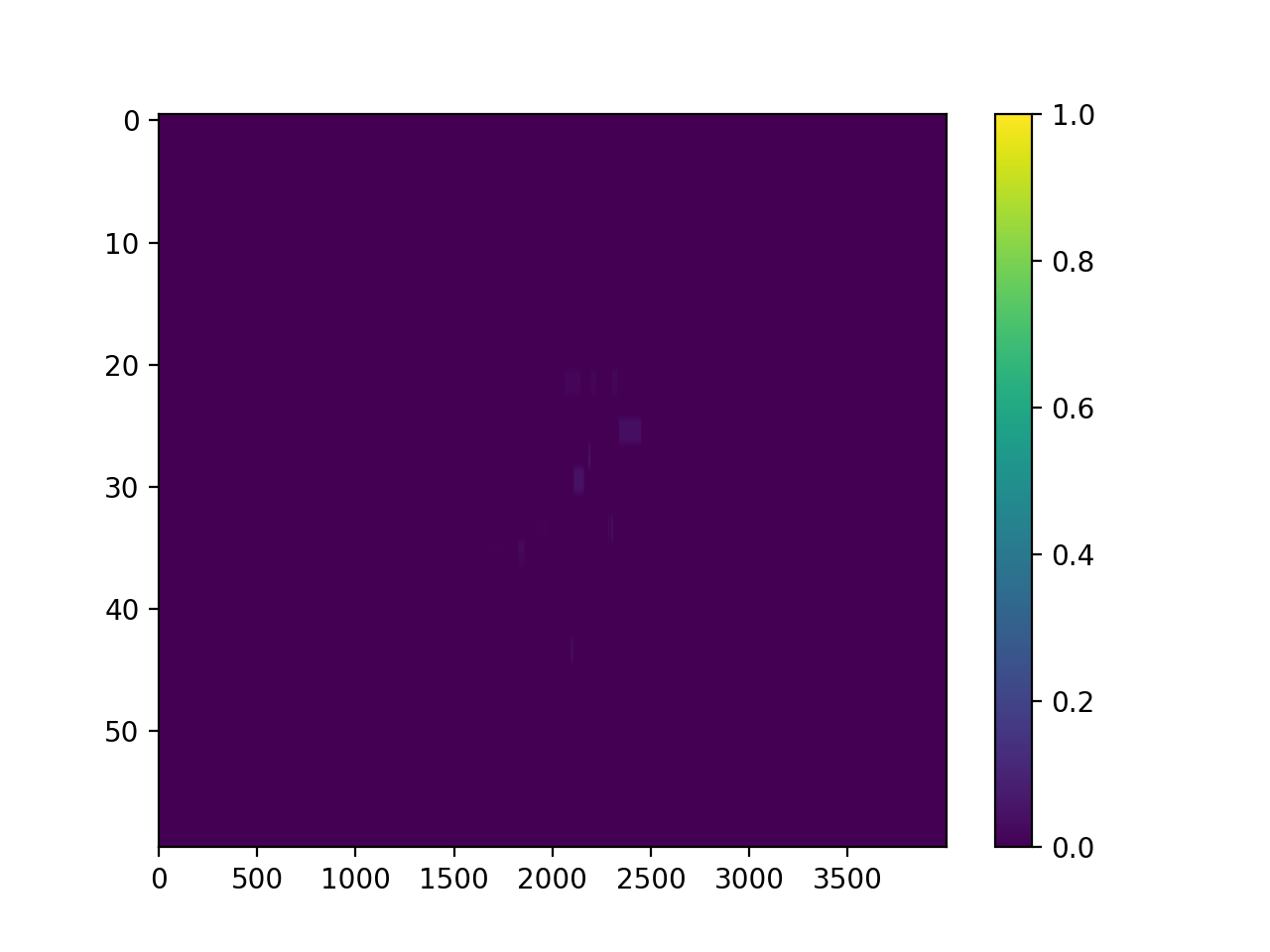
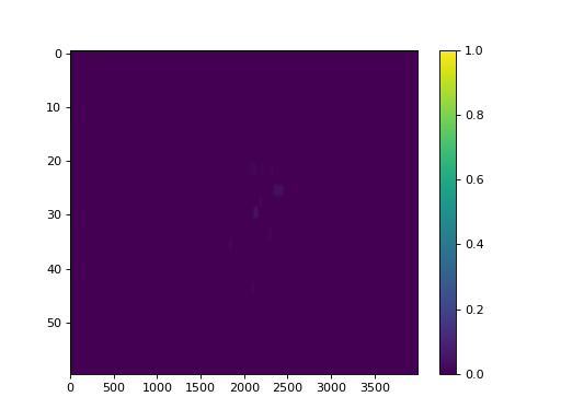
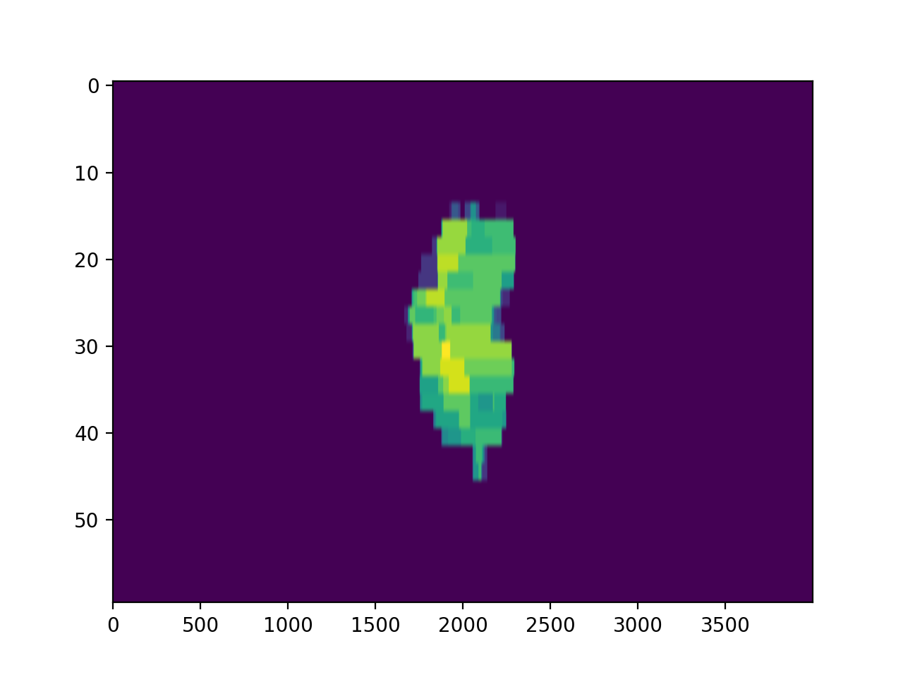
And the fluence gamma. But note we must calculate the gamma first, passing in any DoseTA or DistTA parameters:
log.fluence.gamma.calc_map()
log.fluence.gamma.plot_map()
(Source code, png, hires.png, pdf)
Additionally, you can calculate and view the fluences of subbeams if you’re working with trajectory logs:
log.subbeams[0].fluence.gamma.calc_map()
log.subbeams[0].fluence.actual.plot_map()
(Source code, png, hires.png, pdf)

Converting Trajectory logs to CSV
If you already have the log files, you obviously have a record of treatment. However, trajectory logs are in binary
format and are not easily readable without tools like pylinac. You can save trajectory logs in a more readable format
through the to_csv() method. This will write the log to a comma-separated
variable (CSV) file, which can be read with Excel and many other programs. You can do further or specialized analysis
with the CSV files if you wish, without having to use pylinac:
log = TrajectoryLog.from_demo()
log.to_csv()
Anonymizing Logs
Machine logs can be anonymized two ways. The first is using the anonymize() method, available to
both Trajectory logs and Dynalogs. Example script:
tlog = TrajectoryLog.from_demo()
tlog.anonymize()
dlog = Dynalog.from_demo()
dlog.anonymize()
The other way is the use the module function anonymize(). This function will anonymize a single
log file or a whole directory. If you plan on anonymizing a lot of logs, use this method as it is threaded and is much faster:
from pylinac.log_analyzer import anonymize

log_file = "path/to/tlog.bin"
anonymize(log_file)
log_dir = "path/to/log/folder"
anonymize(log_dir)  # VERY fast
Batch Processing
Batch processing/loading of log files is helpful when dealing with one file at a time is too cumbersome. Pylinac allows you
to load logs of an entire directory via MachineLogs; individual log files can be accessed, and a handful of
batch methods are included.
Example
Let’s assume all of your logs for the past week are in a folder. You’d like to quickly see what the average gamma is of the files:
>>> from pylinac import MachineLogs
>>> log_dir = r"C:\path\to\log\directory"
>>> logs = MachineLogs(log_dir)
>>> logs.avg_gamma(resolution=0.2)
0.03  # or whatever
You can also append to MachineLogs to have two or more different folders combined:
>>> other_log_dir = r"C:\different\path"
>>> logs.append(other_log_dir)
Trajectory logs in a MachineLogs instance can also be converted to CSV, just as for a single instance of TrajectoryLog:
>>> logs.to_csv() # only converts trajectory logs; dynalogs are already basically CSV files
Note
Batch processing methods (like avg_gamma() can take a while if numerous logs have been
loaded, so be patient. You can also
use the verbose=True argument in batch methods to see how the process is going.
API Documentation
Main interface
These are the classes and functions a typical user may interface with.
- pylinac.log_analyzer.load_log(file_or_dir: str, exclude_beam_off: bool = True, recursive: bool = True) TrajectoryLog | Dynalog | MachineLogs[source]
Load a log file or directory of logs, either dynalogs or Trajectory logs.
Parameters
- file_or_dirstr
String pointing to a single log file or a directory that contains log files.
- exclude_beam_offbool
Whether to include snapshots where the beam was off.
- recursivebool
Whether to recursively search a directory. Irrelevant for single log files.
Returns
- One of
Dynalog,TrajectoryLog,
- pylinac.log_analyzer.anonymize(source: str, inplace: bool = False, destination: bool = None, recursive: bool = True)[source]
Quickly anonymize an individual log or directory of logs. For directories, threaded execution is performed, making this much faster (10-20x) than loading a
MachineLogsinstance of the folder and using the.anonymize()method.Note
Because
MachineLoginstances are not overly memory-efficient, you may run intoMemoryErrorissues. To avoid this, try not to anonymize more than ~3000 logs at once.Parameters
- sourcestr
Points to a local log file (e.g. .dlg or .bin file) or to a directory containing log files.
- inplacebool
Whether to edit the file itself, or created an anonymized copy and leave the original.
- destinationstr, None
Where the put the anonymized logs. Must point to an existing directory. If None, will place the logs in their original location.
- recursivebool
Whether to recursively enter sub-directories below the root source folder.
- class pylinac.log_analyzer.Dynalog(filename, exclude_beam_off: bool = True)[source]
Bases:
LogBaseClass for loading, analyzing, and plotting data within a Dynalog file.
Attributes
header :
DynalogHeaderaxis_data :DynalogAxisDatafluence :FluenceStruct- property a_logfile: str
Path of the A* dynalog file.
- property b_logfile: str
Path of the B* dynalog file.
- property num_beamholds: int
Return the number of times the beam was held.
- classmethod from_demo(exclude_beam_off: bool = True)[source]
Load and instantiate from the demo dynalog file included with the package.
- publish_pdf(filename: str, notes: str = None, metadata: dict = None, open_file: bool = False, logo: Path | str | None = None)[source]
Publish (print) a PDF containing the analysis and quantitative results.
Parameters
- filename(str, file-like object}
The file to write the results to.
- notesstr, list of strings
Text; if str, prints single line. If list of strings, each list item is printed on its own line.
- open_filebool
Whether to open the file using the default program after creation.
- metadatadict
Extra data to be passed and shown in the PDF. The key and value will be shown with a colon. E.g. passing {‘Author’: ‘James’, ‘Unit’: ‘TrueBeam’} would result in text in the PDF like: ————– Author: James Unit: TrueBeam ————–
- logo: Path, str
A custom logo to use in the PDF report. If nothing is passed, the default pylinac logo is used.
- static identify_other_file(first_dlg_file: str, raise_find_error: bool = True) str[source]
Return the filename of the corresponding dynalog file.
For example, if the A*.dlg file was passed in, return the corresponding B*.dlg filename. Can find both A- and B-files.
Parameters
- first_dlg_filestr
The absolute file path of the dynalog file.
- raise_find_errorbool
Whether to raise an error if the file isn’t found.
Returns
- str
The absolute file path to the corresponding dynalog file.
- anonymize(inplace: bool = False, destination: str | None = None, suffix: str | None = None) list[str][source]
Save an anonymized version of the log.
For dynalogs, this replaces the patient ID in the filename(s) and the second line of the log with
Anonymous<suffix>. This will rename both A* and B* logs if both are present in the same directory.Note
Anonymization is only available for logs loaded locally (i.e. not from a URL or a data stream). To anonymize such a log it must be first downloaded or written to a file, then loaded in.
Note
Anonymization is done to the log file itself. The current instance of
MachineLogwill not be anonymized.Parameters
- inplacebool
If False (default), creates an anonymized copy of the log(s). If True, renames and replaces the content of the log file.
- destinationstr, optional
A string specifying the directory where the newly anonymized logs should be placed. If None, will place the logs in the same directory as the originals.
- suffixstr, optional
An optional suffix that is added after
Anonymousto give specificity to the log.
Returns
- list
A list containing the paths to the newly written files.
- class pylinac.log_analyzer.TrajectoryLog(filename: str | BinaryIO, exclude_beam_off: bool = True)[source]
Bases:
LogBaseA class for loading and analyzing the data of a Trajectory log.
Attributes
header : ~pylinac.log_analyzer.TrajectoryLogHeader, which has the following attributes: axis_data : ~pylinac.log_analyzer.TrajectoryLogAxisData fluence : ~pylinac.log_analyzer.FluenceStruct subbeams : ~pylinac.log_analyzer.SubbeamManager
- property txt_filename: str
The name of the associated .txt file for the .bin file. The file may or may not be available.
- anonymize(inplace: bool = False, destination: str | None = None, suffix: str | None = None) list[str][source]
Save an anonymized version of the log.
The patient ID in the filename is replaced with
Anonymous<suffix>for the .bin file. If the associated .txt file is in the same directory it will similarly replace the patient ID in the filename withAnonymous<suffix>. Additionally, the Patient ID row will be replaced withPatient ID: Anonymous<suffix>. For v4+ logs, the Patient ID field in the Metadata structure will be replaced withAnonymous<suffix>.Note
Anonymization is only available for logs loaded locally (i.e. not from a URL or a data stream). To anonymize such a log it must be first downloaded or written to a file, then loaded in.
Note
Anonymization is done to the log file itself. The current instance of
MachineLogwill not be anonymized.Parameters
- inplacebool
If False (default), creates an anonymized copy of the log(s). If True, renames and replaces the content of the log file.
- destinationstr, optional
A string specifying the directory where the newly anonymized logs should be placed. If None, will place the logs in the same directory as the originals.
- suffixstr, optional
An optional suffix that is added after
Anonymousto give specificity to the log.
Returns
- list
A list containing the paths to the newly written files.
- classmethod from_demo(exclude_beam_off: bool = True)[source]
Load and instantiate from the demo trajetory log file included with the package.
- to_csv(filename: str | None = None) str[source]
Write the log to a CSV file.
Parameters
- filenameNone, str
If None (default), the CSV filename will be the same as the filename of the log. If a string, the filename will be named so.
Returns
- str
The full filename of the newly created CSV file.
- publish_pdf(filename: str | BinaryIO, metadata: dict = None, notes: str | list = None, open_file: bool = False, logo: Path | str | None = None)[source]
Publish (print) a PDF containing the analysis and quantitative results.
Parameters
- filename(str, file-like object}
The file to write the results to.
- notesstr, list of strings
Text; if str, prints single line. If list of strings, each list item is printed on its own line.
- open_filebool
Whether to open the file using the default program after creation.
- metadatadict
Extra data to be passed and shown in the PDF. The key and value will be shown with a colon. E.g. passing {‘Author’: ‘James’, ‘Unit’: ‘TrueBeam’} would result in text in the PDF like: ————– Author: James Unit: TrueBeam ————–
- logo: Path, str
A custom logo to use in the PDF report. If nothing is passed, the default pylinac logo is used.
- property num_beamholds: int
Return the number of times the beam was held.
- property is_hdmlc: bool
Whether the machine has an HDMLC or not.
- class pylinac.log_analyzer.MachineLogs(folder: str, recursive: bool = True)[source]
Bases:
listRead in machine logs from a directory. Inherits from list. Batch methods are also provided.
Parameters
- folderstr
The directory of interest. Will walk through and process any logs, Trajectory or dynalog, it finds. Non-log files will be skipped.
- recursivebool
Whether to walk through subfolders of passed directory. Only used if
folderis a valid log directory.
Examples
Load a directory upon initialization:
>>> log_folder = r'C:\path\log\directory'
>>> logs = MachineLogs(log_folder)
Batch methods include determining the average gamma and average gamma pass value:
>>> logs.avg_gamma()
>>> 0.05 # or whatever it is
>>> logs.avg_gamma_pct()
>>> 97.2
- classmethod from_zip(zfile: str)[source]
Instantiate from a ZIP archive.
Parameters
- zfilestr
Path to the zip archive.
- property num_logs: int
The number of logs currently loaded.
- property num_tlogs: int
The number of Trajectory logs currently loaded.
- property num_dlogs: int
The number of Trajectory logs currently loaded.
- load_folder(directory: str, recursive: bool = True)[source]
Load log files from a directory and append to existing list.
Parameters
- directorystr, None
The directory of interest. If a string, will walk through and process any logs, Trajectory or dynalog, it finds. Non-log files will be skipped. If None, files must be loaded later using .load_dir() or .append().
- recursivebool
If True (default), will walk through subfolders of passed directory. If False, will only search root directory.
- report_basic_parameters() None[source]
Report basic parameters of the logs.
Number of logs
Average gamma value of all logs
Average gamma pass percent of all logs
- append(obj, recursive: bool = True) None[source]
Append a log. Overloads list method.
Parameters
- objstr, Dynalog, TrajectoryLog
If a string, must point to a log file. If a directory, must contain log files. If a Dynalog or Trajectory log instance, then simply appends.
- recursivebool
Whether to walk through subfolders of passed directory. Only applicable if obj was a directory.
- avg_gamma(doseTA: int | float = 1, distTA: int | float = 1, threshold: int | float = 0.1, resolution: int | float = 0.1) float[source]
Calculate and return the average gamma of all logs. See
calc_map()for further parameter info.
- avg_gamma_pct(doseTA: int | float = 1, distTA: int | float = 1, threshold: int | float = 0.1, resolution: int | float = 0.1) float[source]
Calculate and return the average gamma pass percent of all logs. See
calc_map()for further parameter info.
- to_csv() list[str][source]
Write trajectory logs to CSV. If there are both dynalogs and trajectory logs, only the trajectory logs will be written. File names will be the same as the original log file names.
Returns
- list
A list of all the filenames of the newly created CSV files.
- anonymize(inplace: bool = False, suffix: str | None = None)[source]
Save anonymized versions of the logs.
For dynalogs, this replaces the patient ID in the filename(s) and the second line of the log with ‘Anonymous<suffix>`. This will rename both A* and B* logs if both are present in the same directory.
For trajectory logs, the patient ID in the filename is replaced with Anonymous<suffix> for the .bin file. If the associated .txt file is in the same directory it will similarly replace the patient ID in the filename with Anonymous<suffix>. Additionally, the Patient ID row will be replaced with Patient ID: Anonymous<suffix>.
Note
Anonymization is only available for logs loaded locally (i.e. not from a URL or a data stream). To anonymize such a log it must be first downloaded or written to a file, then loaded in.
Note
Anonymization is done to the log file itself. The current instance(s) of MachineLog will not be anonymized.
Parameters
- inplacebool
If False (default), creates an anonymized copy of the log(s). If True, renames and replaces the content of the log file.
- suffixstr, optional
An optional suffix that is added after Anonymous to give specificity to the log.
Returns
- list
A list containing the paths to the newly written files.
- class pylinac.log_analyzer.Graph(value)[source]
Bases:
Enum- GAMMA = 'gamma'
- HISTOGRAM = 'histogram'
- RMS = 'rms'
Supporting Classes
You generally won’t have to interface with these unless you’re doing advanced behavior.
- class pylinac.log_analyzer.Metadata(stream: BinaryIO, num_axes: int)[source]
Bases:
objectMetadata field for Trajectory logs v4.0+.
Warning
The TrueBeam log file spec says that there is a reserved section of the same size as v3.0 following this section. That is NOT TRUE. It is actually offset by the size of the metadata; meaning 1024 - (64 + num_axes * 8) - 745.
- class pylinac.log_analyzer.Axis(actual: ndarray, expected: ndarray | None = None)[source]
Bases:
objectRepresents an ‘Axis’ of a Trajectory log or dynalog file, holding actual and potentially expected and difference values.
Attributes
Parameters are Attributes
Parameters
- actualnumpy.ndarray
The array of actual position values.
- expectednumpy.ndarray, optional
The array of expected position values. Not applicable for dynalog axes other than MLCs.
- class pylinac.log_analyzer.MLC(log_type, snapshot_idx: ndarray | None = None, jaw_struct=None, hdmlc: bool = False, subbeams=None)[source]
Bases:
objectThe MLC class holds MLC information and retrieves relevant data about the MLCs and positions.
Parameters
- log_type:
Dynalog,TrajectoryLog The log type.
- snapshot_idxarray, list
The snapshots to be considered for RMS and error calculations (can be all snapshots or just when beam was on).
- jaw_struct
JawStruct The jaw structure.
- hdmlcboolean
If False (default), indicates a regular MLC model (e.g. Millennium 120). If True, indicates an HD MLC model (e.g. Millennium 120 HD).
Attributes
- leaf_axesdict containing
Axis The dictionary is keyed by the leaf number, with the Axis as the value.
Warning
Leaf numbers are 1-index based to correspond with Varian convention.
- classmethod from_dlog(dlog, jaws, snapshot_data: ndarray, snapshot_idx: list | ndarray)[source]
Construct an MLC structure from a Dynalog
- classmethod from_tlog(tlog, subbeams, jaws, snapshot_data, snapshot_idx, column_iter)[source]
Construct an MLC instance from a Trajectory log.
- property num_pairs: int
Return the number of MLC pairs.
- property num_leaves: int
Return the number of MLC leaves.
- property num_snapshots: int
Return the number of snapshots used for MLC RMS & Fluence calculations.
Warning
This number may not be the same as the number of recorded snapshots in the log since the snapshots where the beam was off may not be included. See
MachineLog.load()
- property num_moving_leaves: int
Return the number of leaves that moved.
- property moving_leaves: ndarray
Return an array of the leaves that moved during treatment.
- add_leaf_axis(leaf_axis: LeafAxis, leaf_num: int) None[source]
Add a leaf axis to the MLC data structure.
Parameters
- leaf_axisLeafAxis
The leaf axis to be added.
- leaf_numint
The leaf number.
Warning
Leaf numbers are 1-index based to correspond with Varian convention.
- leaf_moved(leaf_num: int) bool[source]
Return whether the given leaf moved during treatment.
Parameters
leaf_num : int
Warning
Leaf numbers are 1-index based to correspond with Varian convention.
- pair_moved(pair_num: int) bool[source]
Return whether the given pair moved during treatment.
If either leaf moved, the pair counts as moving.
Parameters
pair_num : int
Warning
Pair numbers are 1-index based to correspond with Varian convention.
- get_RMS_avg(bank: MLCBank = MLCBank.BOTH, only_moving_leaves: bool = False)[source]
Return the overall average RMS of given leaves.
Parameters
- bank :
Specifies which bank(s) is desired.
- only_moving_leavesboolean
If False (default), include all the leaves. If True, will remove the leaves that were static during treatment.
Warning
The RMS and error will nearly always be lower if all leaves are included since non-moving leaves have an error of 0 and will drive down the average values. Convention would include all leaves, but prudence would use only the moving leaves to get a more accurate assessment of error/RMS.
Returns
float
- get_RMS_max(bank: MLCBank = MLCBank.BOTH) float[source]
Return the overall maximum RMS of given leaves.
Parameters
- bank :
Specifies which bank(s) is desired.
Returns
float
- get_RMS_percentile(percentile: int | float = 95, bank: MLCBank = MLCBank.BOTH, only_moving_leaves: bool = False)[source]
Return the n-th percentile value of RMS for the given leaves.
Parameters
- percentileint
RMS percentile desired.
- bank :
Specifies which bank(s) is desired.
- only_moving_leavesboolean
If False (default), include all the leaves. If True, will remove the leaves that were static during treatment.
Warning
The RMS and error will nearly always be lower if all leaves are included since non-moving leaves have an error of 0 and will drive down the average values. Convention would include all leaves, but prudence would use only the moving leaves to get a more accurate assessment of error/RMS.
- get_RMS(leaves_or_bank: str | MLCBank | Iterable) ndarray[source]
Return an array of leaf RMSs for the given leaves or MLC bank.
Parameters
- leaves_or_banksequence of numbers, {‘a’, ‘b’, ‘both’}
If a sequence, must be a sequence of leaf numbers desired. If a string, it specifies which bank (or both) is desired.
Returns
- numpy.ndarray
An array for the given leaves containing the RMS error.
- get_leaves(bank: MLCBank = MLCBank.BOTH, only_moving_leaves: bool = False) list[source]
Return a list of leaves that match the given conditions.
Parameters
- bank{‘A’, ‘B’, ‘both’}
Specifies which bank(s) is desired.
- only_moving_leavesboolean
If False (default), include all the leaves. If True, will remove the leaves that were static during treatment.
- get_error_percentile(percentile: int | float = 95, bank: MLCBank = MLCBank.BOTH, only_moving_leaves: bool = False) float[source]
Calculate the n-th percentile error of the leaf error.
Parameters
- percentileint
RMS percentile desired.
- bank{‘A’, ‘B’, ‘both’}
Specifies which bank(s) is desired.
- only_moving_leavesboolean
If False (default), include all the leaves. If True, will remove the leaves that were static during treatment.
Warning
The RMS and error will nearly always be lower if all leaves are included since non-moving leaves have an error of 0 and will drive down the average values. Convention would include all leaves, but prudence would use only the moving leaves to get a more accurate assessment of error/RMS.
- create_error_array(leaves: Sequence[int], absolute: bool = True) ndarray[source]
Create and return an error array of only the leaves specified.
Parameters
- leavessequence
Leaves desired.
- absolutebool
If True, (default) absolute error will be returned. If False, error signs will be retained.
Returns
- numpy.ndarray
An array of size leaves-x-num_snapshots
- create_RMS_array(leaves: Sequence[int]) ndarray[source]
Create an RMS array of only the leaves specified.
Parameters
- leavessequence
Leaves desired.
Returns
- numpy.ndarray
An array of size leaves-x-num_snapshots
- leaf_under_y_jaw(leaf_num: int) bool[source]
Return a boolean specifying if the given leaf is under one of the y jaws.
Parameters
leaf_num : int
- get_snapshot_values(bank_or_leaf: MLCBank | Iterable = MLCBank.BOTH, dtype: str = 'actual') ndarray[source]
Retrieve the snapshot data of the given MLC bank or leaf/leaves
Parameters
- bank_or_leafstr, array, list
If a str, specifies what bank (‘A’, ‘B’, ‘both’). If an array/list, specifies what leaves (e.g. [1,2,3])
- dtype{‘actual’, ‘expected’}
The type of MLC snapshot data to return.
Returns
- ndarray
An array of shape (number of leaves - x - number of snapshots). E.g. for an MLC bank and 500 snapshots, the array would be (60, 500).
- log_type:
- class pylinac.log_analyzer.DynalogHeader(dlogdata)[source]
Bases:
StructureAttributes
- versionstr
The Dynalog version letter.
- patient_namestr
Patient information.
- plan_filenamestr
Filename if using standalone. If using Treat =<6.5 will produce PlanUID, Beam Number. Not yet implemented for this yet.
- toleranceint
Plan tolerance.
- num_mlc_leavesint
Number of MLC leaves.
- clinac_scaleint
Clinac scale; 0 -> Varian scale, 1 -> IEC 60601-2-1 scale
- class pylinac.log_analyzer.DynalogAxisData(log, dlogdata)[source]
Bases:
objectAttributes
- num_snapshotsint
Number of snapshots recorded.
- mu
Axis Current dose fraction
Note
This can be gantry rotation under certain conditions. See Dynalog file specs.
- previous_segment_num
Axis Previous segment number, starting with zero.
- beam_hold
Axis Beam hold state; 0 -> holdoff not asserted (beam on), 1 -> holdoff asserted, 2 -> carriage in transition
- beam_on
Axis Beam on state; 1 -> beam is on, 0 -> beam is off
- prior_dose_index
Axis Previous segment dose index or previous segment gantry angle.
- next_dose_index
Axis Next segment dose index.
- gantry
Axis Gantry data in degrees.
- collimator
Axis Collimator data in degrees.
- jaws
Jaw_Struct Jaw data structure. Data in cm.
- carriage_A
Axis Carriage A data. Data in cm.
- carriage_B
Axis Carriage B data. Data in cm.
- mlc
MLC MLC data structure. Data in cm.
Read the dynalog axis data.
- class pylinac.log_analyzer.TrajectoryLogHeader(file: BinaryIO)[source]
Bases:
objectAttributes
- headerstr
Header signature: ‘VOSTL’.
- versionstr
Log version.
- header_sizeint
Header size; fixed at 1024.
- sampling_intervalint
Sampling interval in milliseconds.
- num_axesint
Number of axes sampled.
- axis_enumint
Axis enumeration; see the Tlog file specification for more info.
- samples_per_axisnumpy.ndarray
Number of samples per axis; 1 for most axes, for MLC it’s # of leaves and carriages.
- num_mlc_leavesint
Number of MLC leaves.
- axis_scaleint
Axis scale; 1 -> Machine scale, 2 -> Modified IEC 61217.
- num_subbeamsint
Number of subbeams, if autosequenced.
- is_truncatedint
Whether log was truncated due to space limitations; 0 -> not truncated, 1 -> truncated
- num_snapshotsint
Number of snapshots, cycles, heartbeats, or whatever you’d prefer to call them.
- mlc_modelint
The MLC model; 2 -> NDS 120 (e.g. Millennium), 3 -> NDS 120 HD (e.g. Millennium 120 HD)
- class pylinac.log_analyzer.TrajectoryLogAxisData(log, file, subbeams)[source]
Bases:
objectAttributes
- collimator
Axis Collimator data in degrees.
- gantry
Axis Gantry data in degrees.
- jaws
JawStruct Jaw data structure. Data in cm.
- couch
CouchStruct Couch data structure. Data in cm.
- mu
Axis MU data in MU.
- beam_hold
Axis Beam hold state. Beam pauses (e.g. Beam Off button pressed) are not recorded in the log. Data is automatic hold state. 0 -> Normal; beam on. 1 -> Freeze; beam on, dose servo is temporarily turned off. 2 -> Hold; servo holding beam. 3 -> Disabled; beam on, dose servo is disable via Service.
- control_point
Axis Current control point.
- carriage_A
Axis Carriage A data in cm.
- carriage_B
Axis Carriage B data in cm.
- mlc
MLC MLC data structure; data in cm.
- collimator
- class pylinac.log_analyzer.SubbeamManager(file, header)[source]
Bases:
objectOne of 4 subsections of a trajectory log. Holds a list of Subbeams; only applicable for auto-sequenced beams.
- class pylinac.log_analyzer.Subbeam(file, log_version: float)[source]
Bases:
objectData structure for trajectory log “subbeams”. Only applicable for auto-sequenced beams.
Attributes
- control_pointint
Internally-defined marker that defines where the plan is currently executing.
- mu_deliveredfloat
Dose delivered in units of MU.
- rad_timefloat
Radiation time in seconds.
- sequence_numint
Sequence number of the subbeam.
- beam_namestr
Name of the subbeam.
- property gantry_angle: float
Median gantry angle of the subbeam.
- property collimator_angle: float
Median collimator angle of the subbeam.
- property jaw_x1: float
Median X1 position of the subbeam.
- property jaw_x2: float
Median X2 position of the subbeam.
- property jaw_y1: float
Median Y1 position of the subbeam.
- property jaw_y2: float
Median Y2 position of the subbeam.
- class pylinac.log_analyzer.FluenceStruct(mlc_struct=None, mu_axis: Axis = None, jaw_struct=None)[source]
Bases:
objectStructure for data and methods having to do with fluences.
Attributes
- actual
FluenceBase The actual fluence delivered.
- expected
FluenceBase The expected, or planned, fluence.
- gamma
GammaFluence The gamma structure regarding the actual and expected fluences.
- actual
- class pylinac.log_analyzer.FluenceBase(mlc_struct=None, mu_axis: Axis = None, jaw_struct=None)[source]
Bases:
objectAn abstract base class to be used for the actual and expected fluences.
Attributes
- arraynumpy.ndarray
An array representing the fluence map; will be num_mlc_pairs-x-400/resolution. E.g., assuming a Millennium 120 MLC model and a fluence resolution of 0.1mm, the resulting matrix will be 60-x-4000.
- resolutionint, float
The resolution of the fluence calculation; -1 means calculation has not been done yet.
Parameters
mlc_struct : MLC_Struct mu_axis : BeamAxis jaw_struct : Jaw_Struct
- is_map_calced(raise_error: bool = False) bool[source]
Return a boolean specifying whether the fluence has been calculated.
- calc_map(resolution: float = 0.1, equal_aspect: bool = False) ndarray[source]
Calculate a fluence pixel map.
Image calculation is done by adding fluence snapshot by snapshot, and leaf pair by leaf pair. Each leaf pair is analyzed separately. First, to optimize, it checks if the leaf is under the y-jaw. If so, the fluence is left at zero; if not, the leaf (or jaw) ends are determined and the MU fraction of that snapshot is added to the total fluence. All snapshots are iterated over for each leaf pair until the total fluence matrix is built.
Parameters
- resolutionint, float
The resolution in mm of the fluence calculation in the leaf-moving direction.
- equal_aspectbool
If True, make the y-direction the same resolution as x. If False, the y-axis will be equal to the number of leaves.
Returns
- numpy.ndarray
A numpy array reconstructing the actual fluence of the log. The size will be the number of MLC pairs by 400 / resolution since the MLCs can move anywhere within the 40cm-wide linac head opening.
- class pylinac.log_analyzer.ActualFluence(mlc_struct=None, mu_axis: Axis = None, jaw_struct=None)[source]
Bases:
FluenceBaseThe actual fluence object
Parameters
mlc_struct : MLC_Struct mu_axis : BeamAxis jaw_struct : Jaw_Struct
- class pylinac.log_analyzer.ExpectedFluence(mlc_struct=None, mu_axis: Axis = None, jaw_struct=None)[source]
Bases:
FluenceBaseThe expected fluence object.
Parameters
mlc_struct : MLC_Struct mu_axis : BeamAxis jaw_struct : Jaw_Struct
- class pylinac.log_analyzer.GammaFluence(actual_fluence: ActualFluence, expected_fluence: ExpectedFluence, mlc_struct)[source]
Bases:
FluenceBaseGamma object, including pixel maps of gamma, binary pass/fail pixel map, and others.
Attributes
- arraynumpy.ndarray
The gamma map. Only available after calling calc_map()
- passfail_arraynumpy.ndarray
The gamma pass/fail map; pixels that pass (<1.0) are set to 0, while failing pixels (>=1.0) are set to 1.
- distTAint, float
The distance to agreement value used in gamma calculation.
- doseTAint, float
The dose to agreement value used in gamma calculation.
- thresholdint, float
The threshold percent dose value, below which gamma was not evaluated.
- pass_prcntfloat
The percent of pixels passing gamma (<1.0).
- avg_gammafloat
The average gamma value.
Parameters
- actual_fluenceActualFluence
The actual fluence object.
- expected_fluenceExpectedFluence
The expected fluence object.
- mlc_structMLC_Struct
The MLC structure, so fluence can be calculated from leaf positions.
- calc_map(doseTA: int | float = 1, distTA: int | float = 1, threshold: int | float = 0.1, resolution: int | float = 0.1, calc_individual_maps: bool = False) ndarray[source]
Calculate the gamma from the actual and expected fluences.
The gamma calculation is based on Bakai et al eq.6, which is a quicker alternative to the standard Low gamma equation.
Parameters
- doseTAint, float
Dose-to-agreement in percent; e.g. 2 is 2%.
- distTAint, float
Distance-to-agreement in mm.
- thresholdint, float
The dose threshold percentage of the maximum dose, below which is not analyzed.
- resolutionint, float
The resolution in mm of the resulting gamma map in the leaf-movement direction.
- calc_individual_mapsbool
Not yet implemented. If True, separate pixel maps for the distance-to-agreement and dose-to-agreement are created.
Returns
- numpy.ndarray
A num_mlc_leaves-x-400/resolution numpy array.
- plot_map(show: bool = True)[source]
Plot the fluence; the fluence (pixel map) must have been calculated first.
- histogram(bins: list | None = None) tuple[ndarray, ndarray][source]
Return a histogram array and bin edge array of the gamma map values.
Parameters
- binssequence
The bin edges for the gamma histogram; see numpy.histogram for more info.
Returns
- histogramnumpy.ndarray
A 1D histogram of the gamma values.
- bin_edgesnumpy.ndarray
A 1D array of the bin edges. If left as None, the class default will be used (self.bins).
- plot_histogram(scale: str = 'log', bins: list | None = None, show: bool = True) None[source]
Plot a histogram of the gamma map values.
Parameters
- scale{‘log’, ‘linear’}
Scale of the plot y-axis.
- binssequence
The bin edges for the gamma histogram; see numpy.histogram for more info.
- class pylinac.log_analyzer.JawStruct(x1: HeadAxis, y1: HeadAxis, x2: HeadAxis, y2: HeadAxis)[source]
Bases:
objectJaw Axes data structure.
Attributes
- class pylinac.log_analyzer.CouchStruct(vertical: CouchAxis, longitudinal: CouchAxis, lateral: CouchAxis, rotational: CouchAxis, pitch: CouchAxis | None = None, roll: CouchAxis | None = None)[source]
Bases:
objectCouch Axes data structure.
- class pylinac.log_analyzer.NotALogError[source]
Bases:
OSErrorMachine log error. Indicates that the passed file is not a valid machine log file.
- class pylinac.log_analyzer.NotADynalogError[source]
Bases:
OSErrorDynalog error. Indicates that the passed file is not a valid dynalog file.
- class pylinac.log_analyzer.DynalogMatchError[source]
Bases:
OSErrorDynalog error. Indicates that the associated file of the dynalog passed in (A file if B passed in & vic versa) cannot be found. Ensure associated file is in the same folder and has the same name as the passed file, except the first letter.