Nuclear¶

This module is a re-implementation of the IAEA NMQC toolkit that was written for ImageJ [1], [2]. The toolkit itself appears to be based on the IAEA No. 6 QA for SPECT systems publication [3].

The module is designed as a near drop-in replacement for the ImageJ plugin. The algorithms have been duplicated as closely as possible.

Note

This is not designed to compete or replace the ImageJ plugin. It was designed for RadMachine customers, where Python is available. This should be considered an alternative for those who prefer Python over ImageJ.

In the following examples, the sample images given by the NMQC toolkit are used [4].

Max Count Rate¶

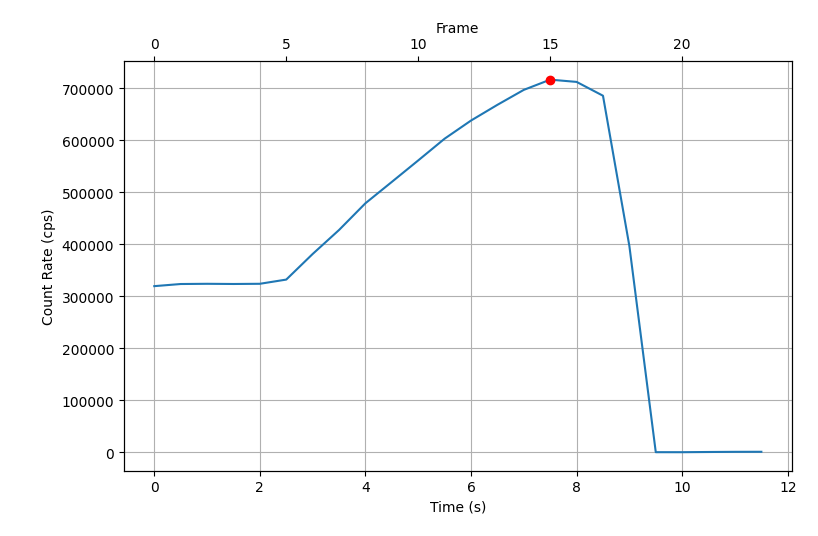
This test is based on the NMQC toolkit and IAEA test 2.3.11.4. The max count rate will examine each frame of a SPECT image and determine the maximum count rate, which is the sum of the pixel values. The maximum count rate and max frame can then be reported. A plot of the count rate vs frame number is also generated.

from pylinac.nuclear import MaxCountRate

path = r"C:\path\to\image.dcm"
mcr = MaxCountRate(path)
mcr.analyze(frame_resolution=0.5)  # or whatever resolution it was acquired at
results = mcr.results_data()
print(results)
mcr.max_countrate  # the maximum count rate
mcr.max_frame  # the frame number of the maximum count rate
mcr.max_time  # the time of the maximum count rate
# plot the count rate vs frame number
mcr.plot()

The plot will look like similar to this:

Planar Uniformity¶

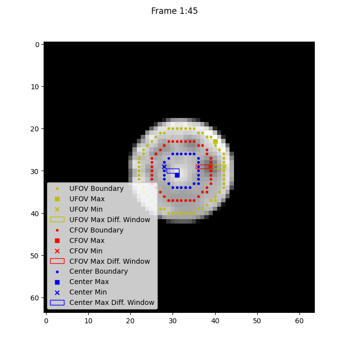
The planar uniformity test is based on test 2.3.3 of the IAEA publication. It will examine each frame of the image and analyze the usable field of view (UFOV) and center field of view (CFOV). Each frame can be plotted to show the UFOV and CFOV, the max points of each, and the sliding window that resulted in the maximum differential uniformity.

Integral Uniformity¶

The integral uniformity uses the same equation as the IAEA, which is the same as the Michelson equation but multiplied by 100. That is:

\[\frac{I_{max} - I_{min}}{I_{max} + I_{min}} \times 100\]

Differential Uniformity¶

The differential uniformity is the same as the IAEA, which is the same as the integral uniformity, but applied to a 5x1 subslice of pixels. The equation is the same as above.

Example Usage¶

from pylinac.nuclear import PlanarUniformity

path = r"C:\path\to\image.dcm"
pu = PlanarUniformity(path)
pu.analyze(ufov_ratio=0.95, cfov_ratio=0.75, window_size=5, threshold=0.75)
results = pu.results_data()
print(results)
pu.plot()  # plot the UFOV and CFOV of each frame

This will result in an image like so:

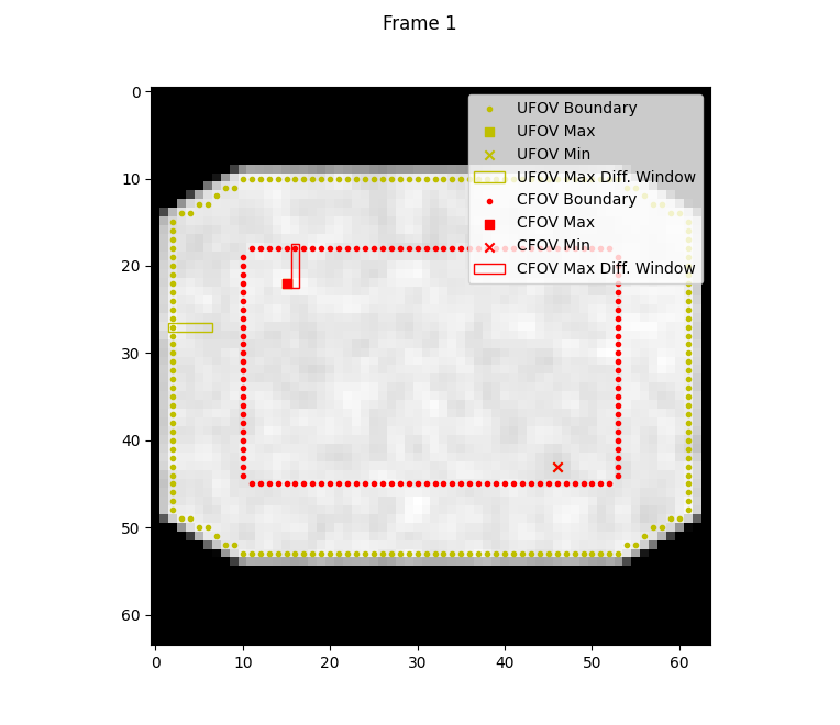
Note the UFOV and CFOV, the min and max pixel values of each FOV, and a rectangle showing the sliding window that resulted in the maximum differential uniformity.

Algorithm¶

The algorithm is largely the same as the NMQC toolkit but there are a few key differences which will be noted in the steps below.

Each step listed here is applied to each frame of the image:

The image is binned to have a pixel size > 4.48mm. I.e. if the pixel size is 1mm, the image will be binned together in a block of 4x4 pixels. The pixels are summed when binned together.
The image is smoothed using a smoothing kernel. The kernel is described on page 59 of the IAEA QC document:

\[\begin{split}\begin{equation} \begin{bmatrix} 1 & 2 & 1 \\ 2 & 4 & 2 \\ 1 & 2 & 1 \end{bmatrix} \end{equation}\end{split}\]

The kernel is normalized by dividing each value by the sum of all values in the kernel.
The edge pixels of the image are set to 0.
The image is thresholded. The threshold is the threshold ratio (input parameter; default of 0.75) multiplied by the mean of all non-zero pixels.

Note

This appears to be up for interpretation. The text says “set any pixels at the edge of the UFOV that contain less than 75% of the mean counts per pixel to zero”. A value of 75% of the mean could mean the entire image; the UFOV is not yet determined at this point. If so, the mean depends on the total FOV. We interpret this to mean a value of 75% of the mean of all pixels that are non-zero.

In practice, this won’t make a big difference since this only affects edge pixels.
Stray pixels are removed from the image. A stray pixel is defined as a pixel that is surrounded ony by pixels of value 0. The stray pixels are set to 0.
The UFOV is determined. The size of the total FOV is found in each dimension (x, y). The UFOV ratio is then multiplied by the total FOV size. This value is then used to “erode” the edge pixel values of the image into a smaller sub-image. E.g. if the total FOV is 22.5cm x 15cm, the UFOV will erode (1-0.95) * 22.5cm = 1.125cm (half of that from each edge).

Note

This appears to be an NMQC-specific implementation. We cannot find anything in the IAEA document that describes this step. The IAEA document only describes the UFOV as the “usable field of view”. The NMQC toolkit appears to differentiate between the total FOV and the UFOV.
The CFOV is determined. The size of the CFOV will be a ratio of the UFOV. E.g. if the UFOV is 20x20cm, the CFOV will be 0.75 * 20cm = 15cm. This difference (5cm in this case) will be “eroded” from the UFOV.
The integral uniformity is calculated for the UFOV and CFOV.
The differential uniformity is calculated for the UFOV and CFOV. The differential uniformity is calculated using a sliding window. The window size is determined by the input parameter window_size. The window size is the number of pixels in the dimension of interest. E.g. if the window size is 5, the window will be 1x5 pixels along the x and y dimensions each. The window is slid across each dimension in 1 pixel increments. The differential uniformity is calculated for each window position. The window position that results in the maximum differential uniformity is recorded.

Note

The NMQC toolkit creates a perfect rectangle for rectangular images. Pylinac will “erode” the image equally in all directions. This will result in images where the corners take on the same shape as the total FOV. Note the clipped corners of the image above for the CFOV. In the case of pylinac, the image shape does not matter and this makes the algorithm easier.

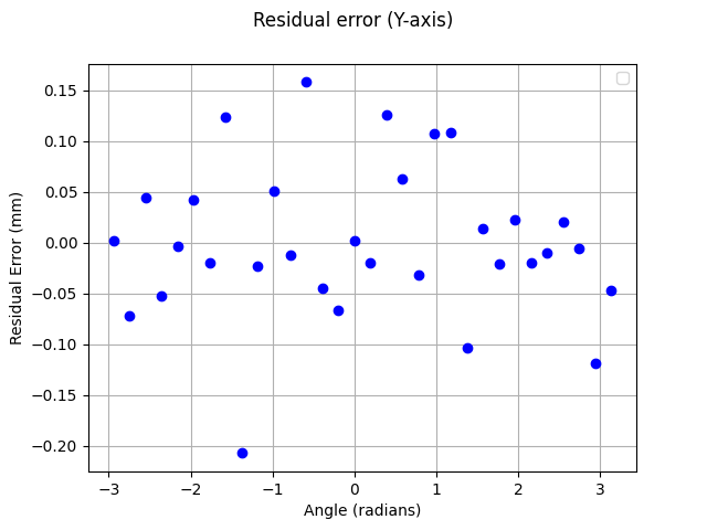
Center of Rotation¶

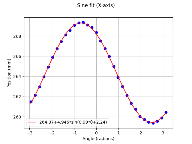
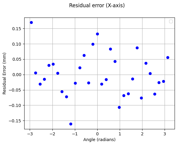
The center of rotation test measures the deviation of the SPECT panel from the center of rotation. I.e. it measures the deviation from an expected orbit. The test is based on the IAEA test 4.3.6, pg 174.

from pylinac.nuclear import CenterOfRotation

path = r"C:\path\to\image.dcm"
cor = CenterOfRotation(path)
cor.analyze()
results = cor.results_data()
print(results)
cor.plot()  # plot the fitted sine x-values, residuals for x and y axis

This will produce a set of plots like so:

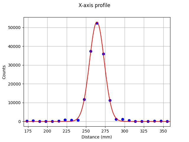
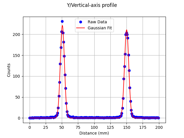
Tomographic Resolution¶

The tomographic resolution test measures the resolution of the SPECT system. The test is based on the IAEA test 4.3.4, pg 169.

from pylinac.nuclear import TomographicResolution

path = r"C:\path\to\image.dcm"
tr = TomographicResolution(path)
tr.analyze()
results = tr.results_data()
print(results)
tr.plot()  # plot the 3 axis profiles and the fitted gaussians

This will produce 3 figures, one for each axis that look like so:

Algorithm¶

The weighted centroid of the entire 3D image stack of frames is calculated.
A 1D profile is created for each axis (x, y, z) at the location of the centroid.
A gaussian is fitted to each profile.
The FWHM and FWTM of each gaussian is calculated.

Note

The FWHM/FWTM is not empirical like it is in the rest of pylinac. It is calculated directly from the gaussian fit per the IAEA publication.

Simple Sensitivity¶

The simple sensitivity test measures the sensitivity of the SPECT system. The test is based on the IAEA test 2.3.8, pg 73. The equations are from the IAEA NMQC toolkit with minor modifications.

Warning

The IAEA NMQC toolkit appears to use the counts of the first frame of the background image only. In the test dataset, the background has 2 frames. Pylinac will use the mean background value of all frames. This will give very small differences in the results if there are multiple frames in the background image.

No background¶

from pylinac.nuclear import SimpleSensitivity, Nuclide

phantom_path = r"C:\path\to\image.dcm"
ss = SimpleSensitivity(path)
ss.analyze(activity_mbq=10, nuclide=Nuclide.Tc99m)
results = ss.results_data()
print(results)

With background¶

from pylinac.nuclear import SimpleSensitivity, Nuclide

phantom_path = r"C:\path\to\image.dcm"
background_path = r"C:\path\to\background.dcm"
ss = SimpleSensitivity(path, background_path=background_path)
ss.analyze(activity_mbq=10, nuclide=Nuclide.Tc99m)
results = ss.results_data()
print(results)

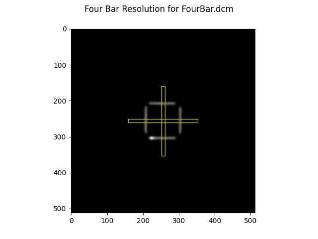
Four-Bar Spatial Resolution¶

The four-bar spatial resolution test measures the spatial resolution of the SPECT system. The test is based on the IAEA test 2.3.8, Method 2, pg 75 and on the NMQC toolkit manual 4.5.3.

from pylinac.nuclear import FourBarResolution

path = r"C:\path\to\image.dcm"
fbr = FourBarResolution(path)
fbr.analyze(separation_mm=100, roi_width_mm=10)
results = fbr.results_data()
print(results)
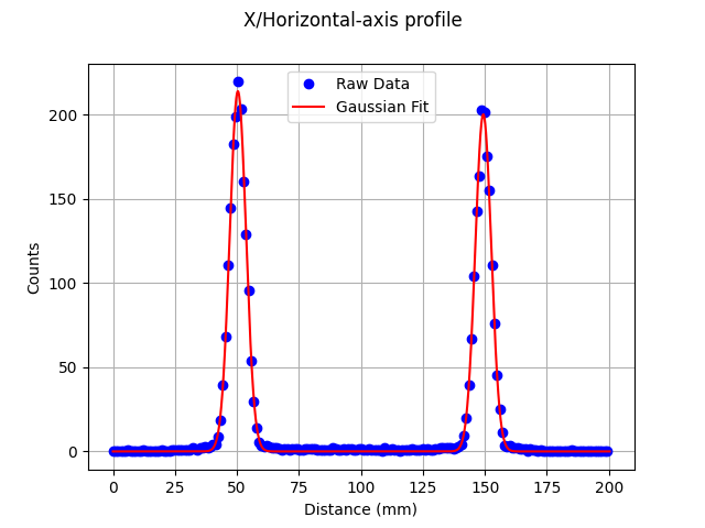
fbr.plot()  # plot the image and 2 axis profiles with fitted gaussians

This will produce a set of plots like so:

Algorithm¶

Warning

The 4 lines are assumed to be centered about the image center.

Note

The image is assumed to only have 1 frame. If there are multiple frames, only the first frame will be used.

2 Rectangular ROIs are sampled. The ROIs are centered at the image center. The longest dimention of the ROI is twice the passed separation_mm. The shortest dimension is the roi_width_mm parameter.
The mean of the profile along the axis of interest is calculated. E.g. for a 100px x 5px this will take a mean across the 5px to give a 100px x 1px profile.
For each axis profile, an initial simple peak search is done to create initial guesses for the gaussian fits.
Each profile is fitted to two gaussian peaks using the initial guesses from the peak search.
The FWHM and FWTM of each gaussian is calculated.
Pixel size (mm/px) is determined by:

\[\frac{Stated Separation}{|G2_{peak} - G1_{peak}|}\]

where \(Stated Separation\) is the separation_mm parameter, \(G1_{peak}\) is the peak position of the first gaussian fit, and \(G2_{peak}\) is the peak position of the second gaussian fit, both in pixels.

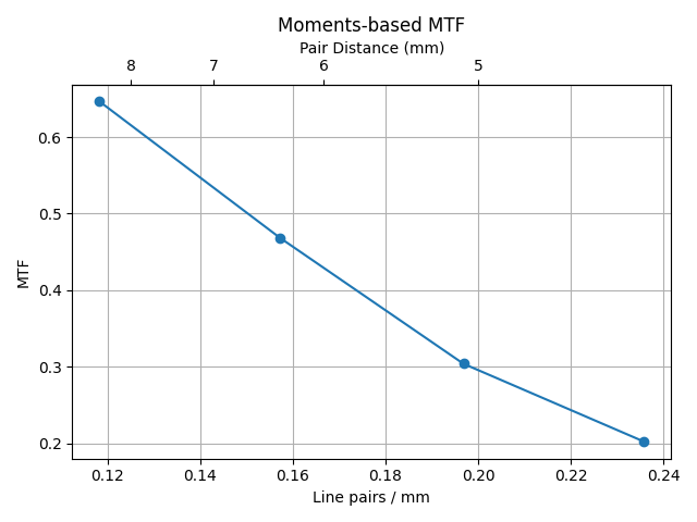
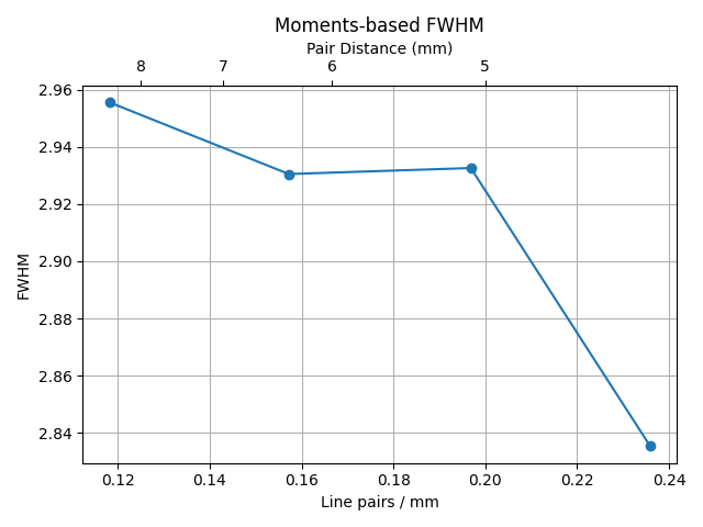
Four-Quadrant Spatial Resolution¶

The four-quadrant spatial resolution test measures the spatial resolution of the SPECT system. The test is based on the IAEA test 2.3.8, Method 2, pg 75 and the NMQC toolkit section 4.5.5.

from pylinac.nuclear import QuadrantResolution

path = r"C:\path\to\image.dcm"
qr = QuadrantResolution(path)
qr.analyze(
    bar_widths=(4.23, 3.18, 2.54, 2.12), roi_diameter_mm=70, distance_from_center_mm=130
)
results = qr.results_data()
print(results)
qr.plot()  # plot the image with quadrant ROIs, the MTF, and the FWHMs.

This will produce a set of plots like so:

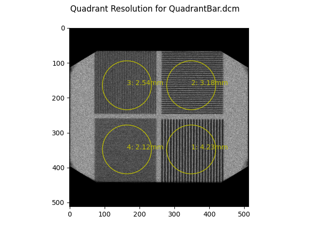
Algorithm¶

Warning

The line pair quadrants are assumed to be equidistant from the image center.

4 circular ROIs are sampled. The ROIs are offset from the image center by distance_from_center_mm. The diameter of the ROI is the roi_diameter_mm parameter. The ROIs start at -45 and go CCW to match the NMQC toolkit.
The mean and standard deviation of each ROI is calculated.
For each ROI, the MTF and FWHM are calculated from Equation 8 and A8 of Hander et al [5]:

(1)¶\[MTF = \frac{\sqrt{2 * (\sigma^{2} - \mu)}}{\mu}\]

(2)¶\[FWHM = 1.058 \times width \times \sqrt{\ln\left(\frac{\mu}{\sqrt{2 \times (\sigma^{2} - \mu)}}\right)}\]

where \(\mu\) is the mean pixel value of the ROI and \(\sigma\) is the standard deviation of the ROI pixel values.

Tomographic Uniformity¶

The tomographic uniformity test measures the uniformity of the SPECT system. The test is based on the IAEA test 4.3.3, pg 165. It is very similar to the Planar Uniformity test.

from pylinac.nuclear import TomographicUniformity

path = r"C:\path\to\image.dcm"
tu = TomographicUniformity(path)
tu.analyze(
    ufov_ratio=0.95,
    cfov_ratio=0.75,
    center_ratio=0.4,
    window_size=5,
    threshold=0.75,
    window_size=5,
)
results = tu.results_data()
print(results)
tu.plot()  # plot the uniformity image, the UFOV, CFOV, and Center ROI, and the sliding windows that resulted in the maximum differential uniformity.

This will result in a plot like so:

Algorithm¶

Note

Compared to the NMQC toolkit, the UFOV, CFOV, and Center ROI are based on ratios of the phantom size and are not absolute. E.g. in the NMQC manual the UFOV is the phantom radius - 2cm and the center ROI is a 6cm circle. These absolute values are not used in pylinac. Instead, ratios are used as are done in the Planar Uniformity test. To get the same results as the NMQC toolkit, basic math from the known phantom size can be used. Further, the default ratios are close to the NMQC toolkit values for the Jaszczak phantom.

The 3D array is sliced to the frames passed by the user.
The mean of the frames of interest are taken along the z-axis (in/out of viewing plane) to create a single 2D image.
From here, the algorithm is the same as the Planar Uniformity test.
In addition to the UFOV and CFOV, a “center” FOV is also sampled based on the center_ratio.
The integral and differential uniformity are calculated for the UFOV, CFOV, and Center ROI.
The center-to-edge ratio is calculated by dividing the mean of the center ROI by the mean value of the pixels between the UFOV and CFOV.

Tomographic Contrast¶

The tomographic contrast test measures the contrast of the SPECT system. The test is based on the IAEA test 4.3.9, pg 182.

from pylinac.nuclear import TomographicContrast

path = r"C:\path\to\image.dcm"
tc = TomographicContrast(path)
tc.analyze(
    sphere_diameters_mm=(38, 31.8, ...),
    sphere_angles=(-10, -70, ...),
    ufov_ratio=0.95,
    search_window_px=5,
    search_slices=3,
)
results = tc.results_data()
print(results)
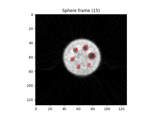
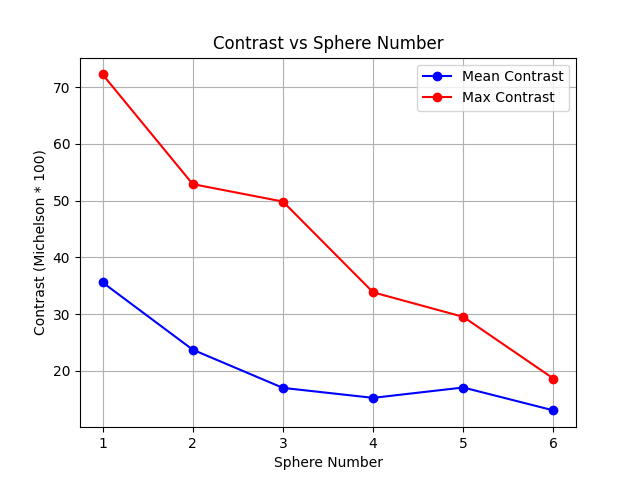
tc.plot()  # plot the image with the ROIs and the contrast values.

This will result in a set of plots like so:

Algorithm¶

Note

Pylinac will automatically identify the uniformity slice and the “sphere” slice. There is no manual option.

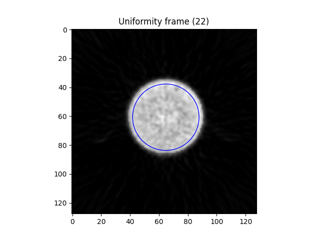
Uniformity Frame¶

The uniformity frame is found by iterating over each frame:
- The frame is thresholded to 10% of the global max pixel value.
- The largest remaining ROI is selected.
- The ROI is eroded by the ufov_ratio parameter (this is similar to what is done for the Planar Uniformity test).
- The uniformity is evaluated for this ROI as well as the ROI diameter, center point, and mean pixel value.
Any frame with an ROI size less than the median - std of all ROI sizes is rejected; this mostly means edge frames are rejected.
The frame with the lowest uniformity is selected as the uniformity frame.

Sphere Frame¶

The initial sphere frame is selected by finding the frame with the highest uniformity (i.e. non-uniformity). This will usually find the slice at or near the spheres as the cold sphere will create non-uniformity.

From this initial sphere frame, each ROI is found by:

Starting at the position indicated by the sphere_angles and sphere_diameters_mm parameters, a minimization is performed to find the best x,y,z coordinates that maximizes the contrast. The search is bounded from the initial position to the search_window_px and search_slices parameters.

Note

The search is in 3D space. However, for ease of plotting, all the sphere ROIs will be shown on one plot when running .plot(). The slice shown will be the most common slice the final sphere locations are determined upon.

References¶

API¶

class pylinac.nuclear.MaxCountRate(path: str | Path)[source]¶

Bases: ResultsDataMixin[MaxCountRateResults]

Calculate the maximum countrate of a gamma camera.

Reimplementation of the NMQC toolkit’s MaxCountRate test (4.2)

Parameters¶

pathstr | Path: The path to the DICOM file.

Parameters¶

ufov_ratiofloat: The ratio of the useful field of view (UFOV) to the detected size of the field of view.
cfov_ratiofloat: The ratio of the central field of view (CFOV) to the UFOV. E.g. if this is 0.75 and the UFOV ratio is 0.95, then the CFOV will be 0.95*0.75=0.7125 of the total FOV.
window_sizeint: The size of the window in pixels to use for the differential uniformity calculation.
thresholdfloat: The threshold to use for removing low-value pixels. This is a fraction of the mean value of the pixels that are > 0.

results() → str[source]¶: Return a string representation of the results.

plot(show: bool = True, cmap: str = 'gray')[source]¶: Plot each frame with the UFOV and CFOV boundaries, max points, and max differential uniformity window.

class pylinac.nuclear.PlanarUniformityResults(*, ufov_integral_uniformity: float, ufov_differential_uniformity: float, cfov_integral_uniformity: float, cfov_differential_uniformity: float)[source]¶

Bases: BaseModel

Create a new model by parsing and validating input data from keyword arguments.

Raises [ValidationError][pydantic_core.ValidationError] if the input data cannot be validated to form a valid model.

self is explicitly positional-only to allow self as a field name.

ufov_integral_uniformity: float¶

ufov_differential_uniformity: float¶

cfov_integral_uniformity: float¶

cfov_differential_uniformity: float¶

model_computed_fields: ClassVar[dict[str, ComputedFieldInfo]] = {}¶: A dictionary of computed field names and their corresponding ComputedFieldInfo objects.

model_config: ClassVar[ConfigDict] = {}¶: Configuration for the model, should be a dictionary conforming to [ConfigDict][pydantic.config.ConfigDict].

model_fields: ClassVar[dict[str, FieldInfo]] = {'cfov_differential_uniformity': FieldInfo(annotation=float, required=True), 'cfov_integral_uniformity': FieldInfo(annotation=float, required=True), 'ufov_differential_uniformity': FieldInfo(annotation=float, required=True), 'ufov_integral_uniformity': FieldInfo(annotation=float, required=True)}¶

Metadata about the fields defined on the model, mapping of field names to [FieldInfo][pydantic.fields.FieldInfo].

This replaces Model.__fields__ from Pydantic V1.

class pylinac.nuclear.CenterOfRotation(path: str | Path)[source]¶

Bases: ResultsDataMixin[CenterOfRotationResults]

Analyze the center of rotation deviation of a gamma camera.

analyze() → None[source]¶: Analyze the DICOM file to determine the deviation from the center of rotation.

property x_cor_deviation_mm: float¶: The deviation of the center of rotation from the center of the matrix in mm.

property y_cor_deviation_mm: float¶: The deviation of the center of rotation from the center of the matrix in mm.

results() → str[source]¶: Return a string representation of the results.

class pylinac.nuclear.CenterOfRotationResults(*, x_deviation_mm: float, y_deviation_mm: float)[source]¶

Bases: BaseModel

Create a new model by parsing and validating input data from keyword arguments.

Raises [ValidationError][pydantic_core.ValidationError] if the input data cannot be validated to form a valid model.

self is explicitly positional-only to allow self as a field name.

x_deviation_mm: float¶

y_deviation_mm: float¶

model_computed_fields: ClassVar[dict[str, ComputedFieldInfo]] = {}¶: A dictionary of computed field names and their corresponding ComputedFieldInfo objects.

model_config: ClassVar[ConfigDict] = {}¶: Configuration for the model, should be a dictionary conforming to [ConfigDict][pydantic.config.ConfigDict].

model_fields: ClassVar[dict[str, FieldInfo]] = {'x_deviation_mm': FieldInfo(annotation=float, required=True), 'y_deviation_mm': FieldInfo(annotation=float, required=True)}¶

Metadata about the fields defined on the model, mapping of field names to [FieldInfo][pydantic.fields.FieldInfo].

This replaces Model.__fields__ from Pydantic V1.

class pylinac.nuclear.TomographicResolution(path: str | Path)[source]¶

Bases: ResultsDataMixin[TomographicResolutionResults]

Analyze a tomographic resolution image for its x/y/z resolution. Based on IAEA test 4.3.4, pg 169

Parameters¶

pathstr | Path: The path to the DICOM file.

analyze() → None[source]¶: Analyze the frames by finding the 3D weighted centroid and then taking a profile of the x/y/z axes and that position

results() → str[source]¶: Return a string representation of the results.

plot()[source]¶: Plot the x/y/z profiles and their gaussian fits.

class pylinac.nuclear.TomographicResolutionResults(*, x_fwhm: float, y_fwhm: float, z_fwhm: float, x_fwtm: float, y_fwtm: float, z_fwtm: float)[source]¶

Bases: BaseModel

Create a new model by parsing and validating input data from keyword arguments.

Raises [ValidationError][pydantic_core.ValidationError] if the input data cannot be validated to form a valid model.

self is explicitly positional-only to allow self as a field name.

x_fwhm: float¶

y_fwhm: float¶

z_fwhm: float¶

x_fwtm: float¶

y_fwtm: float¶

z_fwtm: float¶

model_computed_fields: ClassVar[dict[str, ComputedFieldInfo]] = {}¶: A dictionary of computed field names and their corresponding ComputedFieldInfo objects.

model_config: ClassVar[ConfigDict] = {}¶: Configuration for the model, should be a dictionary conforming to [ConfigDict][pydantic.config.ConfigDict].

model_fields: ClassVar[dict[str, FieldInfo]] = {'x_fwhm': FieldInfo(annotation=float, required=True), 'x_fwtm': FieldInfo(annotation=float, required=True), 'y_fwhm': FieldInfo(annotation=float, required=True), 'y_fwtm': FieldInfo(annotation=float, required=True), 'z_fwhm': FieldInfo(annotation=float, required=True), 'z_fwtm': FieldInfo(annotation=float, required=True)}¶

Metadata about the fields defined on the model, mapping of field names to [FieldInfo][pydantic.fields.FieldInfo].

This replaces Model.__fields__ from Pydantic V1.

class pylinac.nuclear.SimpleSensitivity(phantom_path: str | Path, background_path: str | Path | None = None)[source]¶

Bases: ResultsDataMixin[SimpleSensitivityResults]

The ‘simple’ sensitivity test as defined by IAEA 2.3.9. Equations come from the IAEA NMQC toolkit.

property phantom_cps: float¶: The counts per second of the phantom.

property duration_s: float¶: The duration of the phantom image.

property background_cps: float¶: The counts per second of the background.

results() → str[source]¶: Return a string representation of the results.

property decay_correction: float¶: The decay correction factor.

property sensitivity_mbq: float¶: The sensitivity in MBq.

property sensitivity_uci: float¶: The sensitivity in uCi.

class pylinac.nuclear.SimpleSensitivityResults(*, phantom_cps: float, background_cps: float, half_life_s: float, duration_s: float, decay_correction: float, sensitivity_mbq: float, sensitivity_uci: float)[source]¶

Bases: BaseModel

Create a new model by parsing and validating input data from keyword arguments.

Raises [ValidationError][pydantic_core.ValidationError] if the input data cannot be validated to form a valid model.

self is explicitly positional-only to allow self as a field name.

phantom_cps: float¶

background_cps: float¶

half_life_s: float¶

duration_s: float¶

decay_correction: float¶

sensitivity_mbq: float¶

sensitivity_uci: float¶

model_computed_fields: ClassVar[dict[str, ComputedFieldInfo]] = {}¶: A dictionary of computed field names and their corresponding ComputedFieldInfo objects.

model_config: ClassVar[ConfigDict] = {}¶: Configuration for the model, should be a dictionary conforming to [ConfigDict][pydantic.config.ConfigDict].

model_fields: ClassVar[dict[str, FieldInfo]] = {'background_cps': FieldInfo(annotation=float, required=True), 'decay_correction': FieldInfo(annotation=float, required=True), 'duration_s': FieldInfo(annotation=float, required=True), 'half_life_s': FieldInfo(annotation=float, required=True), 'phantom_cps': FieldInfo(annotation=float, required=True), 'sensitivity_mbq': FieldInfo(annotation=float, required=True), 'sensitivity_uci': FieldInfo(annotation=float, required=True)}¶

Metadata about the fields defined on the model, mapping of field names to [FieldInfo][pydantic.fields.FieldInfo].

This replaces Model.__fields__ from Pydantic V1.

class pylinac.nuclear.FourBarResolution(path: str | Path)[source]¶

Bases: ResultsDataMixin[FourBarResolutionResults]

Spatial resolution in the X and Y direction as measured by a ‘four-bar’ phantom.

Parameters¶

pathstr | Path: The path to the DICOM file.

analyze(separation_mm: float = 100, roi_width_mm: float = 10) → None[source]¶

Take a vertical and horizontal profile about the center of the image.

Fit two gaussians to find the two peaks in each direction.

Parameters¶

separation_mmfloat: The distance between the two peaks in mm. The length of the ROI to sample will be 2x the separation perpendicular to the sample lines.
roi_width_mmfloat: The width of the ROI. This is the width in the direction of the sample lines.

results() → str[source]¶: Return a string representation of the results.

plot(show: bool = True)[source]¶: Plot the image with the sample ROIs and the x/y profiles with gaussian fits

class pylinac.nuclear.FourBarResolutionResults(*, x_fwhm: float, y_fwhm: float, x_fwtm: float, y_fwtm: float, x_measured_pixel_size: float, y_measured_pixel_size: float, x_pixel_size_difference: float, y_pixel_size_difference: float)[source]¶

Bases: BaseModel

Create a new model by parsing and validating input data from keyword arguments.

Raises [ValidationError][pydantic_core.ValidationError] if the input data cannot be validated to form a valid model.

self is explicitly positional-only to allow self as a field name.

model_computed_fields: ClassVar[dict[str, ComputedFieldInfo]] = {}¶: A dictionary of computed field names and their corresponding ComputedFieldInfo objects.

model_config: ClassVar[ConfigDict] = {}¶: Configuration for the model, should be a dictionary conforming to [ConfigDict][pydantic.config.ConfigDict].

model_fields: ClassVar[dict[str, FieldInfo]] = {'x_fwhm': FieldInfo(annotation=float, required=True), 'x_fwtm': FieldInfo(annotation=float, required=True), 'x_measured_pixel_size': FieldInfo(annotation=float, required=True), 'x_pixel_size_difference': FieldInfo(annotation=float, required=True), 'y_fwhm': FieldInfo(annotation=float, required=True), 'y_fwtm': FieldInfo(annotation=float, required=True), 'y_measured_pixel_size': FieldInfo(annotation=float, required=True), 'y_pixel_size_difference': FieldInfo(annotation=float, required=True)}¶

Metadata about the fields defined on the model, mapping of field names to [FieldInfo][pydantic.fields.FieldInfo].

This replaces Model.__fields__ from Pydantic V1.

class pylinac.nuclear.QuadrantResolution(path: str | Path)[source]¶

Bases: ResultsDataMixin[QuadrantResolutionResults]

Analyze a 4-quadrant image of high-contrast line pairs to determine MTF and FWHM.

Parameters¶

pathstr | Path: The path to the DICOM file.

analyze(bar_widths: Sequence[float], roi_diameter_mm: float = 70, distance_from_center_mm: float = 130) → None[source]¶

Analyze the image to determine the MTF resolution and FWHMs.

Parameters¶

bar_widthslist: The bar widths in mm. A line pair will be 2x this value.
roi_diameter_mmfloat: The diameter of the ROI in mm.
distance_from_center_mmfloat: The distance from the center of the image to the center of the ROI in mm.

results() → str[source]¶: Return a string representation of the results.

plot(show: bool = True)[source]¶: Plot the image, the MTF, and the FWHMs.

class pylinac.nuclear.QuadrantResolutionResults(*, quadrants: dict[str, dict[str, float]])[source]¶

Bases: BaseModel

Create a new model by parsing and validating input data from keyword arguments.

Raises [ValidationError][pydantic_core.ValidationError] if the input data cannot be validated to form a valid model.

self is explicitly positional-only to allow self as a field name.

quadrants: dict[str, dict[str, float]]¶: quadrant idx: {‘mtf’: mtf, ‘fwhm’: fwhm, ‘lpmm’: lpmm}

model_computed_fields: ClassVar[dict[str, ComputedFieldInfo]] = {}¶: A dictionary of computed field names and their corresponding ComputedFieldInfo objects.

model_config: ClassVar[ConfigDict] = {}¶: Configuration for the model, should be a dictionary conforming to [ConfigDict][pydantic.config.ConfigDict].

model_fields: ClassVar[dict[str, FieldInfo]] = {'quadrants': FieldInfo(annotation=dict[str, dict[str, float]], required=True)}¶

Metadata about the fields defined on the model, mapping of field names to [FieldInfo][pydantic.fields.FieldInfo].

This replaces Model.__fields__ from Pydantic V1.

class pylinac.nuclear.TomographicUniformity(path: str | Path)[source]¶

Bases: ResultsDataMixin[TomographicUniformityResults], PlanarUniformity

Evaluation of the tomographic uniformity of a SPECT image. Typically, a Jaszczak phantom or similar. This is similar to the Planar Uniformity test.

property frame_result: dict¶: We always have a single result

property frame_key: str¶: The key for the single frame result

center_border_ratio(center_ratio: float, window_size: int) → float[source]¶

The center-to-border ratio as defined by the NMQC toolkit.

The center ROI is a 6cm diameter circle in the center of the phantom. The border ROI is the subtraction of the CFOV from the UFOV.

analyze(first_frame: int = 0, last_frame: int = -1, ufov_ratio: float = 0.8, cfov_ratio: float = 0.75, center_ratio: float = 0.4, threshold: float = 0.75, window_size: int = 5) → None[source]¶

Analyze the image to determine the uniformity. This will take a mean of pixel values for frames between the first and last stated frame.

Parameters¶

first_frameint: The index of the first frame to analyze.
last_frameint: The index of the last frame to analyze.
ufov_ratiofloat: The ratio of the UFOV to the phantom.
cfov_ratiofloat: The ratio of the central FOV to the UFOV.
center_ratiofloat: The ratio of the center ROI to the phantom.
thresholdfloat: The threshold to use for the image.

results() → str[source]¶: Return a string representation of the results.

plot(show: bool = True, cmap: str = 'gray')[source]¶: Plot the image with the sample ROIs

class pylinac.nuclear.TomographicUniformityResults(*, cfov_integral_uniformity: float, cfov_differential_uniformity: float, ufov_integral_uniformity: float, ufov_differential_uniformity: float, center_border_ratio: float, first_frame: int, last_frame: int)[source]¶

Bases: BaseModel

Create a new model by parsing and validating input data from keyword arguments.

Raises [ValidationError][pydantic_core.ValidationError] if the input data cannot be validated to form a valid model.

self is explicitly positional-only to allow self as a field name.

model_computed_fields: ClassVar[dict[str, ComputedFieldInfo]] = {}¶: A dictionary of computed field names and their corresponding ComputedFieldInfo objects.

model_config: ClassVar[ConfigDict] = {}¶: Configuration for the model, should be a dictionary conforming to [ConfigDict][pydantic.config.ConfigDict].

model_fields: ClassVar[dict[str, FieldInfo]] = {'center_border_ratio': FieldInfo(annotation=float, required=True), 'cfov_differential_uniformity': FieldInfo(annotation=float, required=True), 'cfov_integral_uniformity': FieldInfo(annotation=float, required=True), 'first_frame': FieldInfo(annotation=int, required=True), 'last_frame': FieldInfo(annotation=int, required=True), 'ufov_differential_uniformity': FieldInfo(annotation=float, required=True), 'ufov_integral_uniformity': FieldInfo(annotation=float, required=True)}¶

Metadata about the fields defined on the model, mapping of field names to [FieldInfo][pydantic.fields.FieldInfo].

This replaces Model.__fields__ from Pydantic V1.

class pylinac.nuclear.TomographicContrast(path: str | Path)[source]¶

Bases: ResultsDataMixin[TomographicContrastResults]

property uniformity_frame: str¶: The frame with the most uniformity.

analyze(sphere_diameters_mm: Sequence[float] = (38, 31.8, 25.4, 19.1, 15.9, 12.7), sphere_angles: Sequence[float] = (-10, -70, -130, -190, 110, 50), ufov_ratio: float = 0.8, search_window_px: int = 5, search_slices: int = 3) → None[source]¶

Analyze the image to determine the contrast.

Parameters¶

sphere_diameters_mmlist: The diameters of the spheres in mm.
sphere_angleslist: The angles of the spheres in degrees.

results() → str[source]¶: Return a string representation of the results.

plot(show: bool = True)[source]¶: Plot the uniformity frame, sphere ROI frame, and contrast vs sphere number.

class pylinac.nuclear.TomographicContrastResults(*, uniformity_baseline: float, spheres: dict[str, TomgraphicSphere])[source]¶

Bases: BaseModel

Create a new model by parsing and validating input data from keyword arguments.

Raises [ValidationError][pydantic_core.ValidationError] if the input data cannot be validated to form a valid model.

self is explicitly positional-only to allow self as a field name.

model_computed_fields: ClassVar[dict[str, ComputedFieldInfo]] = {}¶: A dictionary of computed field names and their corresponding ComputedFieldInfo objects.

model_config: ClassVar[ConfigDict] = {}¶: Configuration for the model, should be a dictionary conforming to [ConfigDict][pydantic.config.ConfigDict].

model_fields: ClassVar[dict[str, FieldInfo]] = {'spheres': FieldInfo(annotation=dict[str, TomgraphicSphere], required=True), 'uniformity_baseline': FieldInfo(annotation=float, required=True)}¶

Metadata about the fields defined on the model, mapping of field names to [FieldInfo][pydantic.fields.FieldInfo].

This replaces Model.__fields__ from Pydantic V1.

class pylinac.nuclear.Nuclide[source]¶: Bases: object

Nuclear¶

Max Count Rate¶

Planar Uniformity¶

Integral Uniformity¶

Differential Uniformity¶

Example Usage¶

Algorithm¶

Center of Rotation¶

Tomographic Resolution¶

Algorithm¶

Simple Sensitivity¶

No background¶

With background¶

Four-Bar Spatial Resolution¶

Algorithm¶

Four-Quadrant Spatial Resolution¶

Algorithm¶

Tomographic Uniformity¶

Algorithm¶

Tomographic Contrast¶

Algorithm¶

Uniformity Frame¶

Sphere Frame¶

References¶

API¶

Parameters¶

See Also¶

Parameters¶

Parameters¶

Parameters¶

Parameters¶

Parameters¶

Parameters¶

Parameters¶

Parameters¶

Parameters¶